Home Journals Southern Power System Technology
Southern Power System Technology

Abbreviation (ISO4): South Power Sys Technol      Editor in chief:

About  /  Aim & scope  /  Editorial board  /  Indexed  /  Contact  / 
Special Column on Boao New Power System International Forum

Reviewing System Strength Metrics in IBR-Dominated Power Systems: Definitions, Principles, and Classifications

  • Yue ZHU , 1 ,
  • Zitian QIU 2 ,
  • Andreas HADJILEONIDAS 2 ,
  • Yunjie GU 2 ,
  • Tim GREEN 2
Expand
  • 1. Department of Electrical Engineering, City University of Hong Kong, Hongkong 999077, China
  • 2. Department of Electrical and Electronic Engineering, Imperial College London, London SW72AZ, UK

朱越(1993),男,通信作者,助理教授,博士,研究方向为电力系统动态和稳定性分析,;

邱子天(1993),男,博士,研究方向为电力系统暂态稳定;

HADJILEONIDAS Andreas(1999),男,博士研究生,研究方向为电网强度评估。

Received date: 2025-04-29

  Online published: 2025-07-15

Supported by

the City University of Hong Kong Startup Grant for Presidential Assistant Professor(9382007)

the JC STEM Lab of Future Energy Systems(2025⁃0039)

Abstract

Along with the growing integration of renewable energy resources, the new power systems, which are dominated by inverter-based resources (IBRs), are facing critical challenges in both planning and operation stages. The conventionally used system strength metric, short-circuit ratio (SCR), exhibits limitations in assessing connections of new IBRs due to their unique dynamic behaviour and control interactions. In this paper, the definition of system strength is reviewed. The underlying principles of conventional SCR and its variants are then discussed, with their constraints explained. To describe the system strength in a more comprehensive way, this paper further classifies system strength into three categories: quasi-static, small-signal, and large-signal. For each category, relevant metrics are introduced and their relative merits are discussed. Electromagnetic transient simulations are presented to illustrate key insights.

Cite this article

Yue ZHU , Zitian QIU , Andreas HADJILEONIDAS , Yunjie GU , Tim GREEN . Reviewing System Strength Metrics in IBR-Dominated Power Systems: Definitions, Principles, and Classifications[J]. Southern Power System Technology, 2025 , 19(7) : 72 -89 . DOI: 10.13648/j.cnki.issn1674-0629.2025.07.006

0 Introduction

The power system is transforming from a system dominated by synchronous generators(SGs)to a system where inverter-based resources (IBRs) become dominant[1-2]. One consequence is that the system strength, or sometimes known as grid strength,is decreasing in some regions. This is because thermal power plants with synchronous generators are decommissioned in favour of IBRs in the drive to meet the carbon neutrality target[3-4].
Traditionally,short-circuit level(SCL),or short-circuit ratio(SCR)is the standard measure of system strength for indicating the ability to connect a new device at a specific location[5-11].In this context, the new device typically refers to high-voltage direct current(HVDC) systems,which rely on power electronic devices rather than synchronous generators[12-13].A large SCL indicates that a system can provide a large current into a short-circuit(or fault) location and carries an implication that the system is able to hold the system voltage close of nominal value in the face of load variations. It also implies that the system has a low series source impedance,making the system behave more like an ideal voltage source.
However,relying solely on SCL or SCR as a metric presents several challenges in IBR-dominated systems. Firstly,the definition of system strength is vague.It was originally proposed to assess the risk of connecting a new device like HVDC but the concept has been extended to describe system voltage stability[14] and voltage stiffness[15-16]. The widely used SCR has also led to confusion. Sometimes, system strength and SCR are even misused in an interchangeable fashion,i.e.,low‘SCR’means a weak system,and a weak system means low‘SCR’[17].However,the direct link between short-circuit current and system voltage stability remains unclear. Secondly,as synchronous generators(SGs)are replaced by IBRs,particularly grid-following(GFL)IBRs,the conventional representation of the system as an ideal voltage source in series with an impedance becomes inadequate.The GFL IBR behaves like a current source in its normal operation and provides much less fault current contribution due to its tight constraints on over-current.Thirdly,newly connected IBRs may introduce control interactions with existing IBRs,potentially reducing system strength not only at the point of connection but also at other locations where IBRs are already present.Finally,IBRs can introduce instabilities in both small-signal and large-signal(transient)dynamics. Since SCR is analyzed only at the fundamental frequency(50 Hz in China),it fails to capture these characteristics.
To clarify the issues above,this paper reviews the definition of system strength,and analyses the underlying principles of SCR.By identifying the limitations of SCR in IBR-dominated systems and acknowledging that no single metric can describe all characteristics of system strength,this paper classifies system strength into three categories:quasi-static,small-signal,and large-signal.The classification aims to provide a more comprehensive overview of the system strength and offering insights into system behaviour towards different situations.This paper is structured to cover the following topics:
1) How system strength is defined.
2) How SCR is defined,how it is linked to system voltage stability,why it is useful in an SG-dominated system,and why it becomes problematic in IBR-dominated systems.
3) How system strength should be classified.
4) Some newly proposed system strength metrics.
The remainder of the paper is organized as follows:Section 1 introduces the concept of system strength.Section 2 analyses the short circuit ratio (SCR) and its limitations. Section 3 discusses the classifications of system strength. In Section 4,several representative system strength metrics are presented. Section 5 employs electromagnetic transient(EMT)simulations to demonstrate the acquirement of some representative metrics,and provide further insights to these metrics. Finally,Section 6 concludes the paper and discusses potential future work.

1 Understanding System Strength

The traditional understanding of the term ‘strength’of power system is mainly the system ability to connect a new device, which is used in the planning stage[18-19]. Here the new device is typically an HVDC link rather than a new SG.This distinction arises because SGs, with their robust reactive power control via excitation systems,generally do not pose significant connection challenges.In contrast,HVDC links,comprising power electronic devices and controlled by software,operate as constant power sources or loads with strict current constraints.Consequently,assessing whether an HVDC connection could introduce system instabilities becomes a key concern.To address this,SCR,which will be introduced in the next section,has been widely used as a straightforward indicator for evaluating potential stability issues.
With the growing penetration of IBRs,such as wind power plant(WPP),the concept‘strength’is also employed to assess the risk of new IBRs.The term‘system strength’has emerged to encompass a broad range of issues and their implications on power system operability. Explanations of system strength have been made by several system operators and organizations:
1) System strength is a characteristic of an electrical power system that relates to the size of the change in voltage following a fault or disturbance on the power system.⁃AEMC,2017 [16]
2) System strength is the ability of the power system to maintain and control the voltage waveform at any given location in the power system, both during steady state operation and following a disturbance.⁃AEMO,2020 [15]
3) System strength is the ability of power system equipment to operate in a stable manner and for the system as a whole to recover intact from major disturbances.⁃CIGRE,2021 [14]
The above explanations demonstrate that the concept of system strength covers a broad range of system concerns including voltage stiffness,system stability,ability to withstand disturbances and ability to recover from major disturbances.
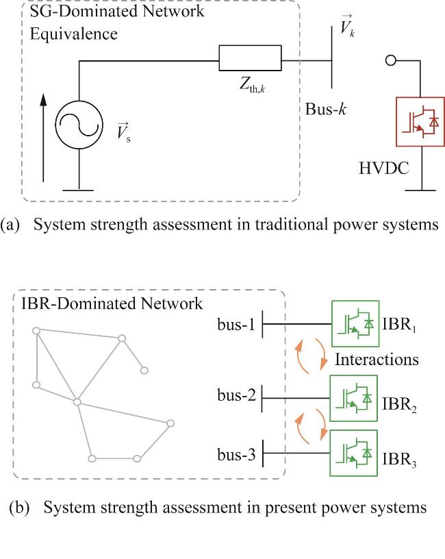
Traditionally,system strength is assessed during the planning stage for a single HVDC connection by representing the grid as an ideal voltage source in series with a Thevenin impedance,as illustrated in Fig.1(a).Under this assumption,the system is linear and does not account for dynamic interactions with the HVDC link. However,with the increasing penetration of IBRs,modern power systems must also consider dynamic interactions among multiple nearby IBRs and the system′s ability to maintain stable operation under such conditions,as depicted in Fig.1(b). Furthermore,the remaining grid itself becomes IBR-dominated,exhibiting nonlinear behavior during large disturbances.These evolving characteristics pose new challenges to conventional system strength assessment methods.
Fig. 1 System strength assessment

2 Short-Circuit Ratio (SCR)

2.1 Principle

The establishment of SCR can be traced back to 1990[5]which is for HVDC system connection study. It was proposed to capture a range of system-level concerns,including high temporary overvoltages,low frequency resonances,risk for voltage/power instability,long restart times and high risk for commutation failures.These concerns were collectively characterized as indicators of system “strength”, and SCR emerged as an aggregate metric for quantifying a system′s ability to withstand such disturbances. Subsequent works[6-11] expanded the SCR concept by formalizing its definition,incorporating fault current analysis,and extending its application to multi-infeed and inverter-based resource(IBR)-dominated systems.Owing to its ease of calculation and ability to reflect multiple concerns,SCR has become a widely adopted metric for assessing system strength. Accordingly,it is important to review its concept and understand the underlying principles.
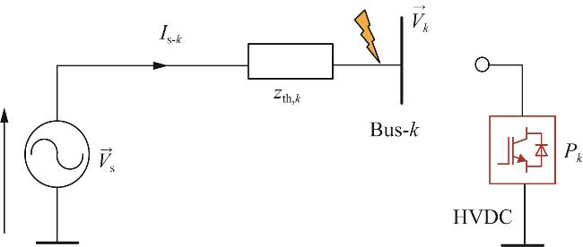
When a system is viewed from a single bus,bus-k in this example,a linearisation can be made on the rest of the system to create an equivalent ideal voltage source in series with a Thevenin impedance, Z t h , k,as shown in Fig.2. Such equivalence is reasonable if the system is dominated by SGs and if the HVDC to be connected is away from the rest of the system. When a three-phase fault is applied at bus-k,i.e.,bus-k is connected to the ground, the power flows from the system to bus-k is defined as the short-circuit capacity (SCC),or SCL,or fault level,and is expressed as
S C C k = V S 2 Z t h , k
Fig. 2 Short-circuit level circuit representation
SCR is then defined as the ratio between SCC and the nominal power of the device connected to bus-k,i.e.,
S C R k = S C C k P k
In a per unit system where the voltage is 1 p.u.,SCR can be expressed in the following equation:
S C R k = 1 Z t h , k , p u ⋅ P k , p u
where Z t h , k , p u and P k , p u represent the Thevenin impedance and device nominal power at bus-k in the per-unit system,respectively. For the sake of brevity,the per unit symbol will be omitted from the following discussion.A global base power is also chosen depending on the scale of the system under consideration.
SCR refers to the ratio between the SCC(the maximum apparent power that the system can supply to this bus during a fault)and the rated power of the device(HVDC in this case)connected to bus-k. An SCR greater than 1 indicates that the systems can supply more current into a short-circuit than the connecting HVDC supplies at full power.

2.2 Understanding

There are two other ways to understand the meaning of SCR,from a view of power transfer and from a view of voltage stability.
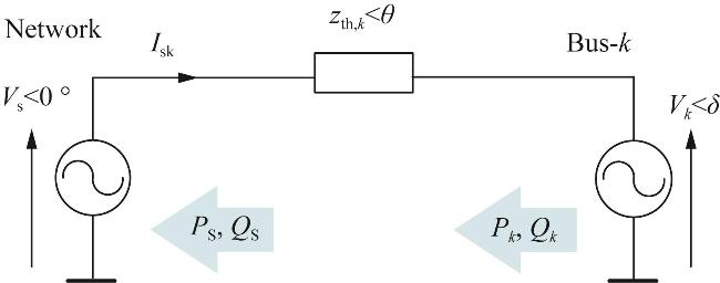
If treating the HVDC at bus-k as a voltage source (which can fix its angle) trying to deliver power to the rest of the system, as shown in Fig.3,it is apparent that when the power angle δ = 90   °,the source approximately reaches the maximum power it can deliver to the system, P M A X , k, which is determined by the Thevenin impedance as
P M A X , k ≈ 1 Z t h , k
Fig. 3 SCR understanding from a power transfer perspective
Substituting (4) into (3) yields
S C R k = P M A X , k P k
Equation (5) shows that SCR is the ratio between the maximum power the system can absorb and the nominal power of the device connected, thus refers to the margin of the power transfer at this bus.
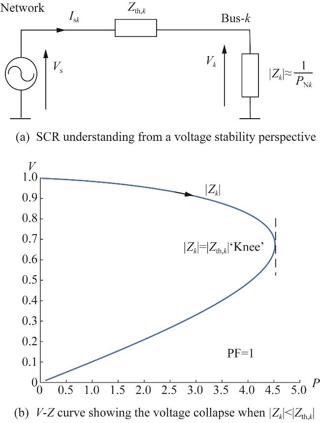
Alternatively,SCR can be understood from a view that a negative load R k,(a negative real part such that it sources current) with power of P k  connected at bus-k and for which the bus voltage must be maintained at around 1 p.u.,as shown in Fig. 4 (a).The magnitude of this impedance can then be expressed as
Z k = 1 P k
Fig. 4 SCR understanding in bus voltage
From circuit principles, it is known that when | Z k | < | Z t h , k |, the voltage at bus-k terminal will collapse, as shown in Fig.4 (b).As a result,the Thevenin impedance of the system sets the minimum magnitude of impedance that the negative load Z k,can have to avoid voltage collapse i.e.,
Z t h , k   = Z k M I N
where | Z k | M I N is the minimum allowed impedance magnitude of the device connected to bus-k.Substituting (6) and (7) into (3) yields
S C R = | Z k | | Z k | M I N
It is seen from (8) that SCR is the ratio between the equivalent impedance of the device when delivering its nominal power and the minimum impedance the system is allowed to connect to maintain the voltage.Accordingly,we also have
S C R = Y k M A X | Y k |
which is the ratio between the maximum allowed admittance for maintaining voltage, Y k M A X,and the equivalent admittance when at the nominal power, | Y k |.A more rigorous proof on the relationship between SCR and system stability can be found in [20],where it is proved that when SCR=1,the rank of system Jacobian matrix becomes 0,and the system is in critical stability state.
From the discussions above,large values of SCR indicate a strong system with a low impedance relative to the connecting device and an expectation of a small variation of voltage magnitude with changes in power flow from this bus.As experience has accumulated,the following judgements can be made based on the value of SCR [21]:
1) When SCR is larger than 5,the system is strong.
2) When SCR is smaller than 5 but larger than 3,the system is weak.
3) When SCR is smaller than 3 but larger than 1,the system is very weak.
4) SCR equalling as 1 is considered as the stability boundary.

2.3 Acquirement of SCR

For a simple circuit where a single device is going to connect to an infinite bus, Z t h , k is directly equal as the line impedance. SCR can then be acquired from equation (3).
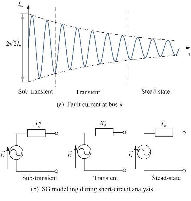
For a meshed network which contains multiple SGs, short-circuit analysis is applied at bus-k to estimate system strength, which can be fulfilled with commercial software tools such as PowerFactory [22].The short-circuit analysis considers a three-phase fault at the point of interaction (POI) and calculates the fault current. There are different methods of short-circuit analysis,e.g.,IEC 60909 method(which excludes loads)[23] and the complete method(which includes loads)[22].As a transient response,the short-circuit current contains three periods:sub-transient, transient,and steady-state period,as demonstrated in Fig.5 (a) [24-25]. Correspondingly, the SG has short-circuit models for each of the period, representing by an ideal voltage source in series with its d-axis sub-transient reactance X d ″,or transient reactance X d ',or steady-state reactance X d, as shown in Fig. 5 (b). Typically, the RMS value of the short-circuit current during the transient period, I k,is applied for system strength assessment.As a result,SCR is essentially a quasi-static indicator.To deal with multiple SGs,superposition method can be applied. The details can be found in [22].
Fig. 5 Short-circuit current in three periods

2.4 Limitations of SCR in IBR-Dominated Systems

Although SCR can be easily acquired from SG-dominated systems via short-circuit analysis and proved useful,the use of SCR in IBR-dominated systems contain certain limitations.
Firstly,short-circuit analysis cannot be directly used to estimate Z t h , k in IBR-dominated systems. From the discussions above,it should be noted that the short-circuit current I k is a way of estimating the Thevenin impedance Z t h , k. Z t h , k can represent system strength while I k itself does not relate to system strength directly.In other words,a small fault current does not necessarily represent a weak system. In an SG-dominated system, Z t h , k can be derived from I k because SG behaves linearly during the fault. However,IBR,especially grid-following IBR,behaves completely differently as SG during a fault. It may be saturated and injecting reactive power of only 1 p.u.,or simply tripped.Consequently,using short-circuit analysis to estimate system strength is not appropriate for an IBR-dominated system.
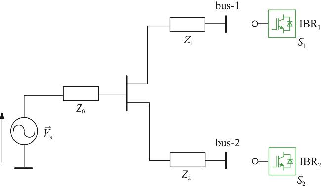
Secondly, SCR cannot capture the interactions among IBRs in the system. With the presence of some control loops,e.g.,phase-locked loop (PLL),IBRs in close proximity may interact with each other,as shown in Fig.1 (b).Typically,the interactions involved will make the system more vulnerable to perturbations,i.e.,weaker. However,such a feature cannot be captured by SCR. This issue can be demonstrated via an example,as shown in Fig.6.
Fig. 6 Two IBRs connecting to the system
Here we consider a simple case where two IBRs in proximity are going to connect to the system,while the main system can still be represented by an SG-dominated system. The rating of the IBRs are S 1 and S 2. Before their connections, SCR at bus-1 and bus-2 can be easily acquired using (3) as
S C R 1 = 1 Z 0 + Z 1 S 1 ,   S C R 2 = 1 Z 0 + Z 2 S 2
It is clear that the calculation of S C R 1 does not consider the existence of IBR2,i.e.,treating it as open circuit. The same assumption applies to S C R 2. Therefore,conventional SCR does not capture any of the interactions among IBRs in the system.
Thirdly,SCR does not capture the system responses to small-perturbations across a range of frequencies,i.e.,small-signal behaviours.As discussed earlier, the estimation of Z t h , k is carried out at the system fundamental frequency (50 Hz in China). This is natural because the impedance at 50 Hz determines the power transfer characteristics. However,the growing penetration of IBRs in the system has brought many dynamics at frequencies other than 50 Hz,especially the sub-synchronous frequencies (below 50 Hz),due to their control-defined behaviour and control interactions among them.These dynamics can produce harmful oscillations in the system. In such cases,system strength assessment must consider whether the connection of an IBR enhances system stability or increases the risk of oscillations.
Lastly,SCR is unable to characterize system responses under large disturbances,such as lightning strikes or short-circuit faults. During such events,the non-linear behaviour and complex control mechanisms of IBRs can lead to situations where the system fails to recover to normal operation after fault clearance.For example,an SCR may enter into saturation during a fault event and unable to exist saturation status immediately when the fault is cleared.Therefore,system strength assessment should account for the system′s capability to recover from large disturbances and the fault ride-through capability of connected IBRs.

3 Classifications of System Strength

To address the limitation that SCR is not a good overall indicator for system strength assessment in IBR-dominated systems,we classify system strength into three categories:quasi-static system strength,small-signal system strength and large-signal system strength,as set out in Table 1. This classification is a natural extension of the system strength explanation introduced in Section 1 and the SCR limitations discussed Section 2.
Tab. 1 Classifications of three new strength metrics
Quasi-static System Strength Small-signal system strength Large-signal system strength
Features

Fundamental frequency analysis (50 Hz)

Using Thevenin equivalence as the major indicator

Small perturbations around an operation point

Frequency-domain analysis (oscillating frequencies)

Large perturbations like faults and voltage sags

Non-linear analysis

Intended Indications

Potential voltage collapse caused by changes of power flow

inadequate voltage regulation

Potential poorly damped oscillations

small-signal interactions among inverters

Excessive recovery time from voltage dips
Existing Metrics

1)CSCR, WSCR, ESCR [21]

2)Voltage sensitivity [26]

3)HMIESCR [19]

4)Site-Dependent SCR (SDSCR) [20]

1)gSCR [27]

2)IMR [28]

3)Grid Strength Impedance Metric

(GSIM) [29]

4)VDSCR[30]

EMT studies
The concept of quasi-static system strength was developed to estimate system strength from a conventional perspective,similarly to SCR,while incorporating the interactions among IBRs.It evaluates the system′s ability to prevent voltage collapse under varying power flow conditions. A key assumption is that the system remains in a steady-state condition at each point during the variation, without accounting for any transient responses,hence using the term‘quasi-static’.Like SCR,quasi-static system strength assesses the Thevenin impedance equivalence at the fundamental frequency,while a major improvement over SCR is that it explicitly considers the influence of nearby IBRs.Existing metrics for quasi-static system strength can be further divided into two groups.The first group includes variants of SCR,including composite short-circuit ratio (CSCR),weighted short-circuit ratio (WSCR),equivalent circuit-based short-circuit ratio (ESCR),and hybrid multi-infeed interactive effective short-circuit ratio (MHIESCR).The second group mainly use voltage sensitivity,i.e., ∂ V ∂ Q.
Small-signal system strength evaluates the system′s dynamic performance in response to small perturbations around the operating point. Specifically,it evaluates the system′s ability to damp oscillations triggered by perturbations introduced at different locations. Unlike quasi-static system strength which is assessed solely at the fundamental frequency,small-signal system strength is evaluated across a range of frequencies in the frequency domain. Existing studies that adopt a frequency domain or small-signal approach include small-signal generalized short-circuit ratio (gSCR),impedance margin ratio (IMR),grid-strength impedance metric (GSIM),and virtual dynamic short-circuit ratio (VDSCR).
Large-signal system strength assesses the system ability to recover to normal following large disturbances,such as local short-circuit faults or deep voltage dips caused by remote faults.Currently,there is no established theoretical method for assessing large-signal system strength. Instead,analysis is typically conducted using EMT simulations,where the non-linear behaviour of IBRs,such as current saturation,must be accurately present.A suitable and widely accepted metric for evaluating large-signal system strength remains unavailable.Therefore,large-signal system strength is not further discussed in this paper.

4 Existing System Strength Metrics

In this section,several recently proposed system strength metrics are reviewed. Given the large number of available metrics,this paper focuses on discussing a selection of the representative ones.

4.1 Quasi-Static System Strength Metrics

Because quasi-static system strength aims to capture the interactions between nearby IBRs, existing metrics, especially the SCR variants, mainly considers cases where multiple IBRs connecting to the same POI via different lines and transformers. Equivalent circuits will be employed to explain their underlaying principles.

1) Composite Short-Circuit Ratio (CSCR)

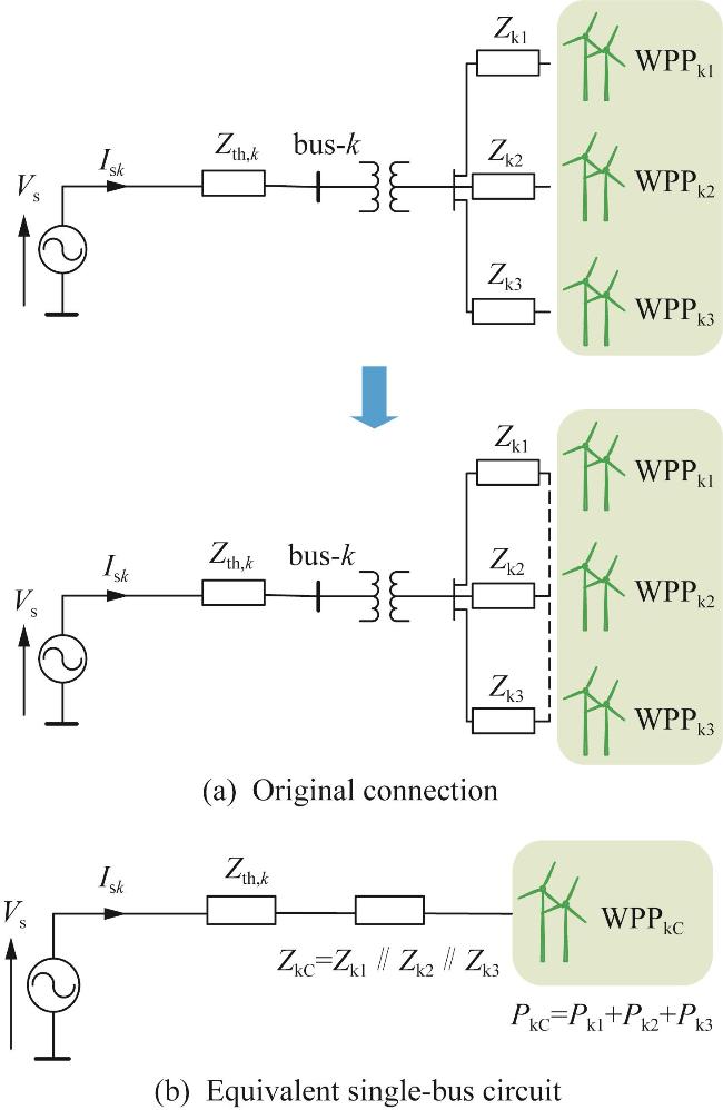
CSCR was proposed by NERC & GE Energy Consulting in 2015 [31]. It addresses scenarios where multiple WPPs are planned to connect to the same high-voltage (HV) bus in the system, as illustrated in Fig. 7 (a), and reaches to a single value as an aggregated system strength. Since each WPP connects to bus k through different line or transformer impedances, their nominal powers cannot simply be summed to form a single aggregated device. Instead, an assumption is made that a common bus is established, to which all WPPs of interest are connected. CSCR is then calculated based on the equivalent circuit as shown in Fig. 7 (b), such that
C S C R = 1 Z t h , k + Z k C P k C
Fig. 7 CSCR illustration
where
Z k C = Z k 1 ∥ Z k 2 ∥ Z k 3 = 1 1 Z k 1 + 1 Z k 2 + 1 Z k 3 ,  
P k C = P k 1 + P k 2 + P k 3 .
As a result, the CSCR reflects the collective impact of the WPPs. If directly assessed SCR at the POI, such that
S C R k = 1 Z t h , k P k C
It is clear from (11) and (12) that CSCR is smaller than SCR k . This reflects the fact that CSCR accounts for the interactions between WPP k 1, WPP k 2 and WPP k 3, leading to a degradation in the overall system strength.

2) Weighted Short-Circuit Ratio(WSCR)

WSCR was proposed by ERCOT in 2014[32]. Similarly to CSCR,WSCR is reflects the collective impact of several WPPs connecting to the same POI. However, unlike CSCR, which assumes each WPP is connected to the POI in a point-to-point manner,WSCR does not consider the actual connection topology.Instead,it first performs a short-circuit analysis at each WPP to acquire the SCC,denoted as SCC ki . It is important to note that when performing the short-circuit analysis at the i-th WPP,all other WPPs are treated as open-circuit,meaning they do not contribute any fault current. WSCR is then calculated by weighting the individual SCC values according to the rated power of each WPP as:
W S C R = ∑ S C C k i × P i ∑ P i 2
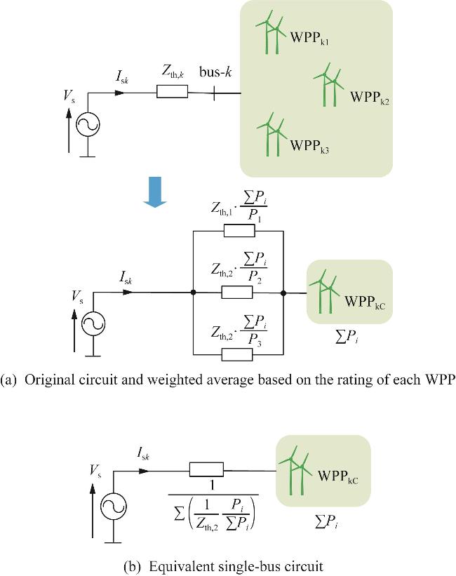
where P i is the nominal power of the device at bus-i. WSCR can be easily acquired from short-circuit analysis in software,while detailed explanation of WSCR was not provided in the original study. As we understand from its equation,WSCR aims to form an equivalent single device to connect to bus-k.A weighted average is carried on the Thevenin impedance seen from each WPP,i.e., Z t h , i based on the corresponding nominal power. After that, a common bus is established,to which all WPPs of interest are connected, as demonstrated in Fig. 8 (a).Due to the parallel connection, a single-bus equivalence can be achieved,as shown in Fig.8 (b). Therefore, WSCR can be represented as
W S C R = 1 Z t h , k W ⋅ ∑ P i
Fig. 8 WSCR illustration
where
Z t h , k W = ∑ P i ∑ P i Z t h , i
It is worth noting that the original Thevenin impedance Z t h , k seen from the POI is merged to the WPP’s Thevenin impedance.For example,for WPP k 1,the Thevenin impedance is
Z t h , 1 = Z t h , k + Z k 1
where Z 1 is the impedance between the WPP and the POI.
Now we compare WSCR with CSCR and traditional SCR. If the topology is the same as in Fig. 7 (a), using the weighting average of WSCR, its Thevenin impedance for a single-bus equivalence is
Z t h , k W = P 1 + P 2 + P 3 P 1 Z t h , k + Z k 1 + P 2 Z t h , k + Z k 2 + P 3 Z t h , k + Z k 3
And for CSCR,
Z t h , k C = Z t h , k + 1 1 Z k 1 + 1 Z k 2 + 1 Z k 3
For a special case where Z k 1 = Z k 2 = Z k 3,
Z t h , k W = Z t h , k + Z k 1
And for CSCR, the aggregated Thevenin impedance is
Z t h , k C = Z t h , k + 1 3 Z k 1
It is clear that Z t h , k < Z t h , k C < Z t h , k W, hence S C R > C S C R > W S C R.
However, both CSCR and WSCR lack a strong theoretical foundation.Although it has been stated that these metrics can capture the interactions between WPPs,it remains unclear how they achieve this. For example,if Z k 1 ,   Z k 2 ,   Z k 3 ≪ Z t h , k,meaning that the WPPs are very close to each other. It is assumed that the interactions between them will be strong,but actually based on (20) it is easy to have C S C R ≈ W S C R   ≈ S C R,leading to an inconsistency:the metrics indicate no difference compared to the conventional SCR,despite the expected strong interactions. Therefore, this paper does not recommend the use of CSCR and WSCR as indicators of quasi-static system strength.

3) Equivalent circuit-based short-circuit ratio (ESCR)

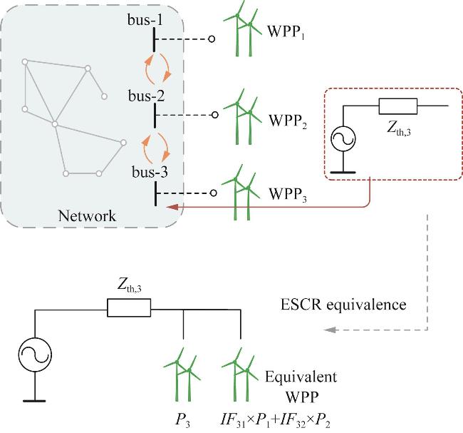
ESCR was proposed by CIGRE in 2016 [21]. The ESCR approach makes use of the observed voltage change at the POI of one WPP bus for a voltage change at the POI of another WPP, as an approximate indicator of the interactions between the WPPs. An interaction factor is defined as
I F i k = Δ V i Δ V k = Z i k Z k k
where Z k k is the self-impedance at bus-i and Z i k is the transfer-impedance between bus-i and bus-k. ESCR is then defined in the following way:
E S C R k = S C C k P k + ∑ i ≠ k I F i k × P i
An illustration of ESCR expressed in the similar format as the other metrics discussed so far is shown Fig.9,where three WPPS connected to bus-1,2,3 which are in close electrical proximity. Strength of bus-3 is then assessed by including the influence from bus-1 and bus-2. In such a case, WPP1 and WPP2 are transferred as an equivalent source at bus-3 through the interaction factor defined in (21). Compared with CSCR and WSCR, ESCR has a clear physical meaning hence is more suitable to capture the interactions between nearby IBRs. Nevertheless, acquiring Z i k may not be straightforward, especially in a meshed network.This process will be demonstrated in the case study.
Fig. 9 ESCR equivalent circuit representation
Another similar metric is the SDSCR proposed by D.Wu et al.[20].Due to its similarity to ESCR,SDSCR is not discussed in details in this paper.

4) Voltage Sensitivity

Using voltage sensitivity, or more accurately,voltage sensitivity to reactive power ∂ V ∂ Q is a straightforward indicator for the bus voltage regulation. Sometimes its reciprocal ∂ Q ∂ V is also applied[26] to align with SCR. Voltage sensitivity considers the fact that the AC voltage of the WPP is maintained by regulating the reactive power. Once ∂ V ∂ Q = 0,the voltage regulation is lost and the system enters into the critical stable point. And once ∂ V ∂ Q < 0,the voltage is collapsed. Compared with SCR,the voltage sensitivity is a metric assessed at the actual power generation,instead of rated power,hence is an on-line assessment. It also reflects the effects of loads,the STACOM,and the control design of IBR. To estimate the voltage sensitivity, an EMT simulation is usually needed.

5) Hybrid Multi-Infeed Interactive Effective Short-Circuit Ratio (HMIESCR)

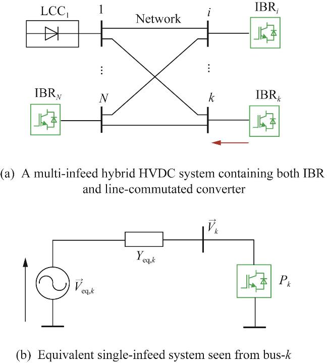
HMIESCR was proposed by Y. Li et al. It aims to assess the system strength in a multi-infeed hybrid HVDC system containing both IBR and line-commutated converter,as shown in Fig.10(a).It first establishes the relationships between voltage and current at all buses:
Δ I = Y ^ Δ V
Fig. 10 Hybrid multi-infeed HVDC system
where Y ^ is the nodal admittance matrix matrix, and Δ V and Δ I are N-demission vector representing variations of voltage and current at each bus.
An equivalent single-infeed circuit is then established from bus-k, as depicted in Fig.10(b). HMIESCR is then defined in the same way as SCR as
H M I E S C R k = V k 2 Y e q , k P k
Using 1 / Z t h , k to replace Y e q , k and taking V k = 1   p . u .,(24) becomes SCR defined in (3).From [19], Y e q , k can be further calculated as
Y e q , k = Y k k - ∑ i = 1 , i ≠ k N Y i k ⋅ M V I F i k
where Y i k is an element in Y ^ and M V I F i k is a multi-infeed voltage interaction factor defined as
M V I F i k = Δ V i Δ V k
Which is a factor representing the ration between changes of voltage at bus-i and bus-k,caused by an output power variation Δ P k.
Substituting (24) to (25) yields
H M I E S C R k = V k 2 Y k k - ∑ i = 1 , i ≠ k N Y i k ⋅ M V I F i k P k
It can be observed from (27) that MHIESCR has a similar format as ESCR defined in (22).Compared with ESCR, one key improvement is that [19] establishes a theorical stability boundary,which is defined as the critical hybrid multi-infeed interactive effective short-circuit ratio(CHMIESCR).By comparing HMIESCR and CHMIESCR,the stability margin can be quantitatively evaluated.Several case studies are also demonstrated in [19].

4.2 Small-Signal System Strength Metrics

The small-signal system strength has been proposed in recent years to capture potential poorly damped oscillations and small-signal interactions between IBRs.To describe the small-signal behaviour,a close-loop frequency-domain impedance/admittance model is usually employed,namely whole-system impedance model or whole-system admittance model.As this modelling approach underpins most of the newly proposed metrics,it will be introduced first. Subsequently,the gSCR and IMR metrics will be presented and briefly analysed.

1) Whole-System Admittance Model

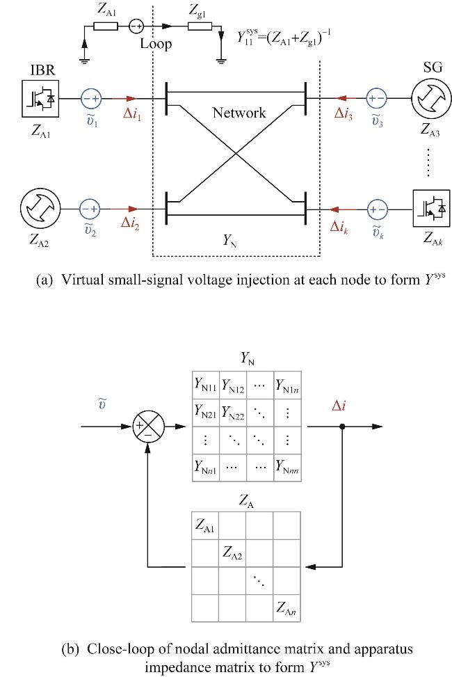
Due to the equivalence between impedance and admittance,we take whole-system admittance Y s y s as an example.It was proposed in [33-34] and is essentially a frequency-domain admittance matrix to describe the dynamic characteristic of the entire system.It chooses the small-signal voltage v ˜ at each POI as the input,equivalent to adding a virtual small voltage perturbation,and the small-signal current Δ i as the output,as shown in Fig.11 (a).
Fig. 11 Formation of whole-system admittance model Y s y s
Y s y s  is then defined as the transfer function from the input to the output,i.e.,
Y s y s ⋅ v = Δ i
It is further proved that through a feedback arrangement as shown in Fig.11 (b), Y s y s can be derived as
Y s y s = I + Y N Z A - 1 Y N
where Y N is the conventional nodal admittance matrix consisting of admittance of branches but extended in frequency domain, Z A is a diagonal impedance matrix where the diagonal entries are the impedances of apparatus at each POI, and I is the identity matrix. The elements of Y s y s are all transfer functions sharing a common set of poles which are also identical to the eigenvalues of the state-space model,i.e.,the criteria that the system maintains stable is that there is no RHP poles for each of the element in Y s y s. It is also worth mentioning that the elements of Y s y s can be monitored through on-line admittance measurement.

2) Generalized Short-Circuit Ratio (gSCR)

gSCR was proposed by H. Xin et al..It was first established at the fundamental frequency to assess the stability margin of a multi-infeed HVDC system [35],and further extended to small-signal perspective to describe the system small-signal stability [27].
gSCR considers the system characteristic equation from (29) that the determinant of the numerators equals 0, such that
d e t   I + Y N Z A = 0
To simplify the equation, gSCR has involved three strong assumptions: i) all IBRs have the same control topology and same parameters, ii) all IBRs are connected through inductors, and iii) the power from the IBR is much less than the line limit. Under such assumptions, (30) can be simplified as
d e t   Y d d s Y d q s Y q d s Y q q s ⊗ I + β s α s - α s β s Y e q = 0
where Y d d s , Y d q s , Y q d s , Y q q s are the IBR admittances in d-q frame, α s and β s are two intermediate quantities. Y e q,which is a n × n matrix, is a newly defined extended admittance matrix and can be derived from
Y e q = S B - 1 B
B is the reduced node susceptance matrix after eliminating passives buses and infinite buses, S B is the power rating of the IBR. Due to the simplification in (31), Y e q is not a transfer function matrix Y e q ( s ),but a numerical matrix at the fundamental frequency, i.e., Y e q ( j ω 0 ). gSCR is then defined as the minimum eigenvalue of Y e q, such that
g S C R ≜ m i n e i g Y e q
gSCR has been shown to be equivalent to the traditional SCR in a single-bus scenario. In multi-bus systems,it can serve as an indicator of overall system stability.
In summary,gSCR extends SCR to multi-bus systems and to small-signal perspective.It is proved to be useful in indicating the system response towards small perturbations.Nevertheless,some strict assumptions are employed,which may limit its applications in IBR-dominated systems.

3) Impedance Margin Ratio (IMR)

Impedance margin ratio (IMR) was proposed by Y.Zhu et al.in [28] as a small-signal system strength metric based on whole-system impedance models.IMR is used to assess the small-signal stability margin at a bus with an IBR connected.A further extension,the admittance margin (AM),was also introduced to evaluate the capability of empty buses to accommodate new IBRs [36].
IMR is defined as the ratio between the maximum allowed variation of the impedance of an IBR and the original value of its impedance at a particular point of interconnection (POI),specifically at the dominant mode λ = σ ± j ω.
Consider a small change added on the impedance of an IBR connected at bus-k,i.e., Δ Z A k.It will lead to a variation of the system eigenvalue Δ λ.It has been proved in [37] that the value of Δ λ can be calculated as
Δ λ = - R e s λ * Y k k s y s ,    Δ Z A k λ
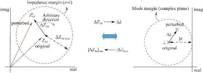
where Y k k s y s is the k-th diagonal element of the whole-system admittance model Y s y s, R e s λ * Y k k s y s refers to the conjugate transpose of the residues of Y k k s y s in d-q frame (a 2 × 2 matrix), Z A k λ is the impedance of the IBR (classed here apparatus to distinguish it from the network) which is connected at bus-k, and the angle bracket refers to the Frobenius inner product. When a strong coupling is found, it is more likely that λ will vary widely for relatively small changes in the apparatus impedance and it is more likely that the mode will move to the right-half plane and become unstable as a result. Such a strong coupling means that the system is‘weak’at this location because the change at this location may lead to system instability. In general, the direction of Δ Z A k and the angle of Δ λ are both unknown. To ensure λ in the left-half plane without knowing the moving direction, the magnitude of ∆λ can be confined to the absolute value of the real part of the existing mode,i.e., Δ λ m a x = σ ,which is considered a mode margin. Correspondingly, Δ Z A k is confined in the range of Z A k m a x,which is called an impedance margin. IMR is then defined as
I M R ≜ Δ Z A k λ M A X Z A k λ = σ - R e s λ * Y k k s y s ⋅ Z A k λ
which is the ratio between the margin of impedance variation and the magnitude of the original impedance. The principle of IMR is illustrated in Fig. 12.
Fig. 12 IMR illustration on complex plane, at s=λ. The change of local apparatus impedance will lead to a change of mode λ, while the maximum mode variation circle (blue dashed circle) then determines the range of allowable impedance variation (red dashed circle) [28]
Based on the analyses,this new metric processes the following merits:
1) IMR is analyzed in the frequency domain,especially at the oscillatory frequency of a mode of concern. IMR points to an observable poorly damped oscillatory mode at the POI with a specific stability margin.
2) IMR is a localised value indicating the small-signal system strength at the POI being considered and hence it can be used to pinpoint weak areas in the system.
3) IMR is calculated from the whole-system admittance model which naturally reflects the interactions among multiple apparatuses in a multi-infeed system.
It is also proved in [28] that at the fundamental frequency,
S C R = 1 1 - I M R
Through a set of case studies, it is pointed out that IMR<0.1 refers to a very weak system, meaning that changes at this location can easily cause significant and long-lasting oscillations and can propagate to the entire system.

4) Virtual Dynamic Short-Circuit Ratio (VDSCR)

VDSCR was proposed by X. Zhang et al. as a small-signal system strength. It aims to convert the stability margin of the IBR plant under different working conditions to a rated single IBR unit, thus providing a simple way of estimating the small-signal system strength and providing guidance in IBR design.
For a n parallel inverter system which is similar to Fig. 7 (a), and assuming that all inverters have the same control structure and parameters, VDSCR is defined as
V D S C R = k - 1 Y g Y B - 1
where k is a virtual coefficient which transfers the inverters with different rated power to a unified rated power. Y g is the grid admittance and is considered as simply an inductance in [30]. Y B is defined as
Y B = V n 2 P n
where P n and V n are the rated power of a single inverter and the bus voltage. The threshold of VDSCR can also be acquired based on phase margin analysis.
Compared with gSCR and IMR,VDSCR can be applied when the system is unstable.However,VDSCR is established based on two conditions:all IBRs have the same control parameters and algorithms,and the rest of the network does not contain any dynamics.These conditions may not be achievable in IBR-dominated power systems.

5 Case Study

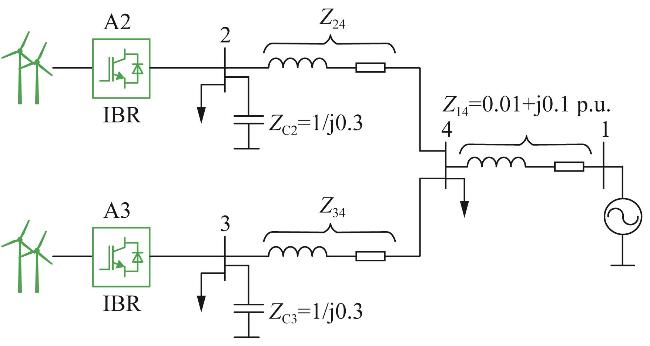
A 4-bus system with one SG and two IBRs is established to demonstrate the assessment of system strength,as shown in Fig.13.The two IBRs,A2 and A3,are configured as grid-following inverters equipped with PLL. Each IBR delivers 0.32 p.u.active power to the system.
Fig. 13 Single-line diagram of the 4-bus test system
The detailed system data including IBR parameters is available in [38].SCR,ESCR and IMR are selected as representatives of traditional metric,quasi-static system strength metric,and small-signal system strength metric. Two case studies featuring the same system structure but different IBR control parameters are presented to illustrate:(i) the limitations of SCR,(ii) how ESCR accounts for interactions among IBRs,and (iii) how IMR characteristics the system′s small-signal behaviour.

5.1 Case 1

In the first case,A2 and A3 are well tuned well with a current control bandwidth of 1 500 Hz and PLL bandwidth of 10 Hz. The line impedance Z 24 and Z 34 are set as 0.02+0.2j p.u..For simplicity,the SG is treated as an ideal voltage source.Therefore,for the Thevenin impedance, taking Z t h , 2 as an example,can be calculated as
Z t h , 2 = Z 14 ∥ Z 34 + Z C 3 + Z 24 ∥ Z C 2 = 0.037 + j 0.333 .
And therefore SCR is
S C R 2 = S C R 3 = 1 Z t h , 2 = 9.3202 ,
which represents a strong system.
Unlike SCR which excludes the influence of A3 when calculating SCR2,ESCR treats both A2 and A3 as two sources.First,by considering each bus having a current injection source,we have a nodal admittance matrix Y n o d a l as
Y n o d a l = Y 14 Y c 2 + Y 24 - Y 14 - Y 24 - Y 14 - Y 24 Y c 3 + Y 34 - Y 34 - Y 34 10 - 6 ,
which is well-used in power flow calculation. The elements in Y n o d a l are admittance of each component, e.g., Y 14 = Z 14 - 1. It is worth noting that bus-4 has no device connected, and hence should be eliminated for ESCR assessment. According to the node elimination principle, we can have
Y r e d n o d a l = Y [ 1 : 3,1 : 3 ] n o d a l - Y 1 : 3,4 n o d a l Y 4,4 n o d a l - 1 Y 4,1 : 3 n o d a l ,
where Y r e d n o d a l becomes a 3 × 3 matrix. By calculating the inverse of Y r e d n o d a l, we have the nodal impedance matrix
Z = Y r e d n o d a l - 1 .
Substituting the elements of Z into (21) yields the interaction factor I F 23 = I F 32 = 0.347   2.And finally,substituting the value of Z t h , 2 and I F 23 into (22) yields E S C R 2 = E S C R 3 = 6.918   1. The value of ESCR is smaller than SCR,indicating a degradation of quasi-static system strength when considering the IBR interaction but is still large enough.
For IMR calculation,the whole-system impedance,or whole-system admittance should be acquired.This can be fulfilled either from an on-line identification process by injecting small perturbations [39],or using existing differential equations. Since the analytical model is available in this case,the mode λ = σ ± j ω, Y s y s ,and Z A k can be acquired,which leads to IMR from (35). In this case, I M R 2 = I M R 3 = 0.655   1, which is away from the threshold 0.1.Hence the small-signal system strength is considered enough.

5.2 Case 2

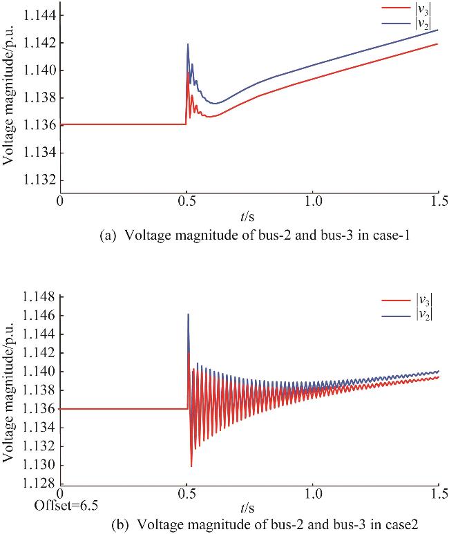
In this case,the network structure remains unchanged,while the control parameters of A2 and A3 are modified by increasing the bandwidth of their PLLs from 5 Hz to 50 Hz for A2 and 30 Hz for A3. The higher PLL bandwidth enhances the small-signal interactions between A2 and A3,as the two grid-following IBRs become more sensitive to voltage perturbations.Since the network configuration is unchanged,both SCR and ESCR remain the same. However,IMR successfully captures the increased interactions.Specifically,the results show I M R 2 = 0.087   1,and I M R 3 = 0.090   5,indicating very weak system conditions at both locations,with A2 being slightly weaker due to its higher PLL bandwidth. The system strength assessment results are demonstrated in Table 2.Fig.14 presents the voltage magnitude waveforms of v 2 and v 3 during a -50% load step change at bus-2 in time-domain simulations. It can be observed that there are minimal oscillations during the transient period in Case 1,which aligns with the system strength assessment indicating that bus-2 and bus-3 are strong.In contrast,significant oscillations are observed in Case 2,indicating a weak system seen from bus-2 and bus-3,and IMR successfully captures this characteristic.These results show that,compared with SCR,ESCR provides an improved estimation of system strength by considering the interactions between IBRs. However,for a more precise assessment of small-signal behaviour,IMR proves to be a better choice.
Tab. 2 SCR, ESCR and IMR in different cases
Case Line impedance/p.u. PLL bandwidth/Hz SCR ESCR IMR
Case1 A2 0.02+j0.2 5 9.320 2 6.918 1 0.655 1
A3 0.02+j0.2 5 9.320 2 6.918 1 0.655 1
Case2 A2 0.02+j0.2 50 9.320 2 6.918 1 0.087 1
A3 0.02+j0.2 30 9.320 2 6.918 1 0.090 5
Fig. 14 Voltage magnitude during a -50% load step at bus-2

6 Conclusions and Future Work

This paper reviews the definition of system strength and its extended interpretation in IBR-dominated power systems. The traditional system strength metric,Short-Circuit Ratio (SCR),is analysed in depth,and its limitations,particularly in systems with high IBR penetration,are highlighted. To better capture the evolving characteristics of modern power systems,system strength is further classified into three categories:quasi-static system strength,small-signal system strength,and large-signal system strength. The concept,physical meaning,and intended indication of each category are discussed to provide a clearer understanding of their respective roles in system analysis. It is also pointed out that an appropriate and widely accepted metric for large-signal system strength is still absent.Developing suitable models that can capture the nonlinear dynamics of IBRs under large disturbances remains an open research challenge.
Several recently proposed metrics,including CSCR,WSCR,ESCR,and voltage sensitivity for quasi-static system strength,are introduced and critically analysed.Their advantages and limitations in practical application are discussed.While these metrics provide improved insights compared to traditional SCR,each comes with its own assumptions and constraints.For small-signal system strength,the metrics gSCR and IMR are reviewed. It is shown that although gSCR can represent overall system stability to some extent,it lacks the ability to capture control interactions between IBRs and provide locational information.IMR,on the other hand,offers a more detailed and sensitive assessment of small-signal behaviour at specific points of interconnection. Finally,a 4-bus,2-IBR test system is employed to demonstrate the application of selected metrics under different operating scenarios.It shows that traditional metrics like SCR and ESCR can give an estimation of system strength,but more refined metrics like IMR are necessary to accurately assess small-signal stability,especially when considering the dynamic interactions between IBRs.
While several new metrics have been proposed to assess the system strength of IBR-dominated power systems,further work is needed in several key areas.First,the extensions of SCR,e.g.,ESCR, lacks clear numerical benchmarks.Currently,values of ESCR do not offer a well-established interpretation. More rigorous justification and clarification of ESCR thresholds are required. Second,deriving small-signal system strength metrics such as gSCR,IMR,GSIM often involves multiple steps and complex impedance identification processes.Simplified assessment methods or user-friendly tools are thus desirable.Furthermore,appropriate IBR models for large-signal system strength assessment remains to be developed. And last,most existing studies overlook the role of system loads,especially constant power loads,which significantly impact stability and should be explicitly included in future assessments.

[13] TAKIDDIN A, ISMAIL M, ZAFAR U, et al. Deep autoencoder-based anomaly detection of electricity theft cyberattacks in smart grids[J]. IEEE Systems Journal, 2022, 16(3): 4106 - 4117.

[14] ROELOFS C M A, GÜCK C, FAULSTICH S. Transfer learning applications for autoencoder-based anomaly detection in wind turbines[J]. Energy and AI, 2024(17): 100373.1 - 100373.10.

[15] LEI L, WU B, FANG X, et al. A dynamic anomaly detection method of building energy consumption based on data mining technology[J]. Energy, 2023( 263): 125575.1 - 125575.19.

[16] YIN S, YANG H, XU K, et al. Dynamic real⁃time abnormal energy consumption detection and energy efficiency optimization analysis considering uncertainty[J]. Applied Energy, 2022(307): 118314.1 - 118314.15.

[17] ZHANG J, CHENG L, YANG Z, et al. An enhanced semi-supervised learning method with self-supervised and adaptive threshold for fault detection and classification in urban power grids[J]. Energy and AI, 2024( 17): 100377.1 - 100377.15.

[18] HE K, FAN H, WU Y, et al. Momentum contrast for unsupervised visual representation learning[A/OL]. arXiv, 2020[2025 - 05 - 24].http://arxiv.org/abs/1911.05722.

[19] CHEN T, KORNBLITH S, NOROUZI M, et al. A simple framework for contrastive learning of visual representations[Z/OL]. arXiv, 2020[2025 - 05 - 24].

[20] CHEN X, HE K. Exploring simple siamese representation learning[Z/OL]. arXiv, 2020[2025 - 05 - 24].http://arxiv.org/abs/2011.10566.

[21] CHEN H, GUO L, BAO W, et al. Extraction of high-resolution air conditioning load profiles from low-resolution smart meter: a semi-supervised nonintrusive approach[J]. IEEE Transactions on Industrial Informatics, 2024, 20(6): 8294 - 8305.

[22] GAO A, MEI F, ZHENG J, et al. Electricity theft detection based on contrastive learning and non-intrusive load monitoring[J]. IEEE Transactions on Smart Grid, 2023, 14(6): 4565 - 4580.

[23] MA D, LIU Z, GAO Q, et al. Few-shot fault diagnosis of EHA based on MTF-ResNet-MA and dual-attribute adaptive decision-level fusion[J]. Measurement, 2025(247): 116787.1 - 116787.12.

[24] MOHAMMADI F N, MILLER L, TAN C W, et al. Deep learning for time series classification and extrinsic regression: a current survey[J]. ACM Computing Surveys, 2024, 56(9): 217:1 - 217:45.

[25] GOSWAMI M, CHALLU C, CALLOT L, et al. Unsupervised model selection for time-series anomaly detection[A/OL]. arXiv, 2023[2025 - 05 - 22].http://arxiv.org/abs/2210.01078.

[26] ZHANG K, WEN Q, ZHANG C, et al. Self-supervised learning for time series analysis: taxonomy, progress, and prospects[J]. IEEE Transactions on Pattern Analysis and Machine Intelligence, 2024, 46(10): 6775 - 6794.

[27] DEHAYBE H, CATANZARO D, CHEVALIER P. Deep reinforcement learning for inventory optimization with non-stationary uncertain demand[J]. European Journal of Operational Research, 2024, 314(2): 433 - 445.

[28] Smartmeter energy consumption data in london households -london datastore[EB/OL]. [2025 - 05 - 24].https://data.london.gov.uk/dataset/smartmeter-energy-use-data-in-london-households.

[29] GHORBANI R, REINDERS MJT, TAX DMJ. PATE: proximity-aware time series anomaly evaluation[A/OL]. arXiv, 2024[2025 - 05 - 27].http://arxiv.org/abs/2405.12096.

[1]
BLAABJERG F, CHEN Z, KJAER S B.Power electronics as efficient interface in dispersed power generation systems[J]. IEEE Transactions on Power Electronics, 2004, 19(5):1184 - 1194.

[2]
GU Y, GREEN T C. Power system stability with a high penetration of inverter-based resources[J]. Proceedings of the IEEE, 2022(1): 356 - 367.

[3]
International Energy Agency (IEA). Global energy review 2021[R/OL]. (2021) [2025 - 04 - 10]. https://www.iea.org/reports/global-energy-review-2021/renewables.

[4]
HATZIARGYRIOU N, MILANO F, AJJARAPU V, et al. Definition and classification of power system stability – Revisited & extended[J]. IEEE Transactions on Power Systems, 2021, 36(4): 3271 - 3281.

[5]
FRANKEN B, ANDERSSON G. Analysis of HVDC converters connected to weak AC systems[J]. IEEE Transactions on Power Systems, 1990, 5(1): 235 - 242.

[6]
GAVRILOVIC A. AC/DC system strength as indicated by short circuit ratios[C]//International Conference on AC and DC Power Transmission, May 5 - 6, 1991, London, UK. New York: IEEE, 1991: 27 - 32.

[7]
DAMANIK O, SAKINCI Ö C, GRDENIĆ G, et al. Evaluation of the use of short-circuit ratio as a system strength indicator in converter-dominated power systems[C]//2022 IEEE PES Innovative Smart Grid Technologies Conference Europe (ISGT-Europe), November 12 - 14, 2022, Novi Sad, Serbia. New York: IEEE, 2022: 1 - 5.

[8]
NIMPITIWAN N, HEYDT G T, AYYANAR R, et al. Fault current contribution from synchronous machine and inverter based distributed generators[J]. IEEE Transactions on Power Delivery, 2007, 22(1): 634 - 641.

[9]
LIU Y, CHEN Z. Short circuit ratio analysis of multi-infeed HVDC system with a VSC-HVDC link[C]//IECON 2011 - 37th Annual Conference of the IEEE Industrial Electronics Society, April 24 - 25, Melbourne, Australia. New York:IEEE, 2011: 949 - 954.

[10]
North American Electric Reliability Corporation (NERC). Integrating inverter-based resources into low short circuit strength systems: Reliability guideline[R]. USA, 2017[2025 - 04 - 10]. https://www.nerc.com/comm/RSTC_Reliability_Guidelines.

[11]
YAMADA Y, TSUSAKA A, NANAHARA T, et al. A study on short-circuit-ratio for an inverter-based resource with power-voltage curves[J]. IEEE Transactions on Power Systems, 2024, 39(4): 6076 - 6086.

[12]
IEEE. IEEE guide for planning DC links terminating at AC locations having low short-circuit capacities: IEEE Standard 1204 - 1997 [S]. New York: IEEE, 1997.

[13]
GONZALEZ J W, WEINDL C, HEROLD G, et al. Feasibility of HVDC for very weak AC systems with SCR below 1.5[C]//Proceedings of the 12th International Power Electronics and Motion Control Conference, May 23 - 25, Portoroz, Slovenia. New York: IEEE, 2006: 1522 - 1527.

[14]
BADRZADEH B, EMIN Z, GOYAL S, et al. System strength[J]. CIGRE Science & Engineering, 2021(N20): 5 - 27.

[15]
Australian Energy Market Operator (AEMO). System strength in the NEM explained[R/OL]. Australia, 2020[2025 - 04 - 10]. https://aemo.com.au/-/media/files/electricity/nem/system-strength-explained.pdf.

[16]
Australian Energy Market Commission (AEMC). National electricity amendment (managing power system fault levels) Rule 2017 [S].Australia: Australian Energy Market Commission (AEMC), 2017.

[17]
GORDON S, BELL K, HONG Q. Implications of reduced fault level and its relationship to system strength: a Scotland case study[C]//CIGRE Session 2022, August 28- September 2, 2022, Paris, France. Paris: CIGRE,2022 : Paper C 4 - 10204_2022.

[18]
National Grid ESO. Provision of short circuit level data[R/OL]. 2022[2025 - 04 - 10]. https://www.nationalgrideso.com/document/238741/download.

[19]
XIAO H, ZHANG Y, DUAN X, et al. Evaluating strength of hybrid multi-infeed HVDC systems for planning studies using hybrid multi-infeed interactive effective short-circuit ratio[J]. IEEE Transactions on Power Delivery, 2020, 8977(c): 1 - 1.

[20]
WU D, LI G, JAVADI M, et al. Assessing impact of renewable energy integration on system strength using site-dependent short circuit ratio[J]. IEEE Transactions on Sustainable Energy, 2018, 9(3): 1072 - 1080.

[21]
CIGRE. Connection of wind farms to weak AC networks[R/OL]. Paris: CIGRE, 2016[2025 - 04 - 10]. https://e-cigre.org/publication/671-connection-of-wind-farms-to-weak-ac-networks.

[22]
DIgSILENT. Short-circuit analysis[M]//PowerFactory technical reference documentation. Chapter 26.

[23]
International Electrotechnical Commission. Short-circuit currents in three-phase AC systems - part 0: calculation of currents: IEC 60909 - 0 [S]. London, IEC, 2016.

[24]
DE METZ-NOBLAT B, DUMAS F, POULAIN C. Calculation of short-circuit currents[J]. Cahier Technique, 2005(158): 124 - 135.

[25]
North American Electric Reliability Corporation. Short-circuit modeling and system strength white paper[R/OL]. New York: North American Electric Reliability Corporation, 2018[2025 - 04 - 10].

[26]
LUND T, WU H, SOLTANI H, et al. Operating wind power plants under weak grid conditions considering voltage stability constraints[J]. IEEE Transactions on Power Electronics, 2022, 37(12): 15482 - 15492.

[27]
DONG W, XIN H, WU D, et al. Small signal stability analysis of multi-infeed power electronic systems based on grid strength assessment[J]. IEEE Transactions on Power Systems, 2019, 34(2): 1393 - 1403.

[28]
ZHU Y, GREEN T C, ZHOU X, et al. Impedance margin ratio: a new metric for small-signal system strength[J]. IEEE Transactions on Power Systems, 2024, 39(6): 7291 - 7303.

[29]
HENDERSON C, EGEA-ALVAREZ A, KNEUPPEL T, et al. Grid strength impedance metric: an alternative to SCR for evaluating system strength in converter dominated systems[J]. IEEE Transactions on Power Delivery, 2024, 39(1): 386 - 396.

[30]
XIAO Y, ZHANG X, ZHAN X, et al. Design-oriented small-signal stability assessment of grid-following inverter-based resources based on virtual dynamic short-circuit ratio[J]. IEEE Transactions on Industrial Electronics, 2019, 1(2): 432 - 445.

[31]
GE Energy Consulting, Midcontinent Independent System Operator (MISO). Minnesota renewable energy integration and transmission study (final report)[R/OL]. 2014[2025 - 04 - 10]. http://mn.gov/commerce-stat/pdfs/mrits-report-2014.pdf.

[32]
ZHANG Y, HUANG S H F, SCHMALL J, et al. Evaluating system strength for large-scale wind plant integration[C]//2014 IEEE PES General Meeting, November 11 - 15, 2014, National Harbor, MD, USA. New York: IEEE, 2014: 1 - 5.

[33]
GU Y, LI Y, ZHU Y, et al. Impedance-based whole-system modeling for a composite grid via embedding of frame dynamics[J]. IEEE Transactions on Power Systems, 2021, 33(2):1231 - 1242.

[34]
ZHU Y, GU Y, LI Y, et al. Impedance-based root-cause analysis: Comparative study of impedance models and calculation of eigenvalue sensitivity[J]. IEEE Transactions on Power Systems, 2022, 15(1): 567 - 583.

[35]
ZHANG F, XIN H, WU D, et al. Assessing strength of multi-infeed LCC-HVDC systems using generalized short-circuit ratio[J]. IEEE Transactions on Power Systems, 2019, 34(1): 467 - 480.

[36]
HADJILEONIDAS A, ZHU Y, GREEN T C. Admittance margin: A guideline for placement of grid-following and grid-forming inverters regarding small-signal stability[C]//IECON 2024, February 10 - 13, 2024, Chicago, IL, USA. New York: IEEE, 2024: 1 - 6.

[37]
ZHU Y, GU Y, LI Y, et al. Participation analysis in impedance models: the grey-box approach for power system stability[J]. IEEE Transactions on Power Systems, 2022, 37(1): 343 - 353.

[38]
Simplus Grid Tool[CP/OL]. 2025[2025 - 04 - 10]. https://github.com/Future-Power-Networks/Simplus-Grid-Tool/tree/2023Mar14_SmallSignalStrength.

[39]
ZHU Y, GU Y, DÖHLER J S, et al. Hybrid data/model-driven whole-system admittance identification via single-point injections[EB/OL]. TechRxiv, 2025 - 03 - 28.

Outlines

/

〈 〉