Home Journals Electric Power
Electric Power

Abbreviation (ISO4): Electric Power      Chairperson: Changyu OUYANG

About  /  Aim & scope  /  Editorial board  /  Indexed  /  Contact  / 
Original article

Price-quantity curve construction strategy for wind-storage power plants participating in the day-ahead spot market

  • Chu QI , 1, 2 ,
  • Yilin LI 1 ,
  • Siyao DU 3 ,
  • Fanpeng ZENG 4 ,
  • Xianmin MU 1 ,
  • Quan LV , 1 ,
  • Zhiqiang WANG 1
Expand
  • 1 School of Electrical Engineering, Dalian University of Technology, Dalian 116024, China
  • 2 State Grid Zhejiang Electric Power Co., Ltd.Hangzhou Xiaoshan Power Supply Company, Hangzhou 311200, China
  • 3 Dalian Power Supply Company of State Grid Liaoning Electric Power Co., Ltd., Dalian 116000, China
  • 4 Jiangsu Lin Yang Energy Co., Ltd., Qidong 226200, China

Received date: 2026-04-07

  Revised date: 2026-06-25

  Online published: 2026-09-03

Supported by

National Key Research and Development Program of China(2025YFA1017900)

Abstract

In the context where wind-storage power plants are gradually participating in the electricity spot market under the "both quantity and price bidding"mode,this paper studies the decision-making problem of constructing price-quantity curves for wind-storage combined systems in the day-ahead energy market.Comprehensively considering the uncertainties of wind power output and electricity prices,energy storage lifetime degradation costs,and market rule constraints,a stochastic optimization model aimed at maximizing expected revenue is established.The model simulates the uncertainties of wind power output and market prices using the scenario method and generates optimal hourly price-quantity curves using a mixed-integer linear programming approach.Case study results show that the proposed model can effectively improve the market revenue performance of wind-storage power plants.Compared with the traditional"quantity-only bidding"mode,the price-quantity curve bidding strategy demonstrates significant advantages in reducing uncertainty costs and optimizing economic benefits.Furthermore,increasing the number of bidding segments significantly promotes revenue enhancement. The research results provide scientific decision support for the market-oriented operation of wind-storage power plants.

Cite this article

Chu QI , Yilin LI , Siyao DU , Fanpeng ZENG , Xianmin MU , Quan LV , Zhiqiang WANG . Price-quantity curve construction strategy for wind-storage power plants participating in the day-ahead spot market[J]. Electric Power, 2026 , 59(8) : 194 -204 . DOI: 10.11930/j.issn.1004-9649.202604017

0 引言

随着"双碳"战略目标的推进,风电的渗透率持续攀升  [1] 。然而,风力发电所固有的随机性、波动性及反调峰特性给电力系统的实时平衡与安全稳定运行带来了巨大挑战  [2] 。为了平滑风电出力波动,提升其可控性与可预测性,近年来"风电+储能"的联合运行模式在政策驱动下快速发展。多地区明确规定,新建风电场须按要求配置一定比例的储能设施方可并网,这为风储电站的推广应用提供了制度保障  [3]
为促进新能源消纳与发展,电力市场化改革不断深化,风储电站参与市场的模式正经历着重要转型,正在逐步由"报量不报价"模式转变为"报量报价"模式。在这一新型市场模式下,作为市场主体的风储电站,需要向市场运营机构申报其在不同价格下的电力供应意愿,即量价曲线。量价曲线的制定直接决定其在现货市场中的出清电量,进而决定其市场化收益。因此,如何构建量价曲线已成为风储电站参与现货市场的核心问题。
当前报量报价决策研究主要集中于火电机组,其常采用多阶段框架来简化优化过程  [4-8] 。然而,新能源发电具有高度不确定性和零边际成本特性,有限储能容量会带来弱可控性和时段间的强耦合性。这与具有明确发电成本和高度可控性的火力发电存在显著差异,导致现有报价策略难以直接移植适用。
而在风储电站参与现货电能量市场方面,现有研究已较为广泛。然而,多数研究基于新能源报量不报价的市场规则展开,重点研究新能源电站优化运营  [9-13] 、不确定性建模  [14-18] 与多市场协同优化  [19-24] 等问题,对于新能源电站在报量报价规则下量价曲线构建策略的研究较少。文献[25]构建了一种考虑风电出力、电价不确定性及决策者风险偏好的水风联合现货市场竞价模型,验证了水风联合竞价在提高收益和降低风险方面的有效性,但其重点关注水风联合竞价的互补效应与决策者风险偏好的影响,对量价曲线的构建机理并未深人分析。文献[26]提出了一种考虑风电预测误差的日前量价阶梯曲线报价策略,通过建立双层优化模型来划分出力区间并优化报价,从而减少偏差惩罚并提升风电场收益,但忽略了储能系统在当前电力市场中提升风电站市场收益的巨大潜力,其算例中将储能排除在现货市场参与之外,与风电普遍配储的行业趋势不符。文献[27]提出了一种考虑碳交易的风光储场站双层报价策略模型,通过电-碳耦合报价和储能协同调控,实现了现货市场收益最大化与系统碳排放降低的双重目标,但主要关注碳交易影响下的风光储协同调控与双层市场出清,对于风光储电站日前市场量价曲线的具体构建策略和动态调整机制分析较少。文献[28]对风电、光伏和储能的发电成本进行排序,依据风电、光伏的发电成本构建了两段式量价曲线,并将边际成本较高的储能作为调节资源,但忽略了申报多段量价曲线对适应风电、光伏波动性的重要价值。
综上,现有研究虽为风储电站参与电力市场提供了重要基础,但对于"报量报价"模式下,如何构建量价曲线,协同优化其分段价格、功率,以实现储能平抑风电发电不确定性与峰谷电价套利双重效益最大化的研究尚不深入。为此,本文聚焦于风储电站参与日前电能量市场的量价曲线构建决策问题展开研究。首先分析了风储电站参与日前电能量市场决策的关键问题;然后构建以各时段量价曲线的分段价格与功率长度为决策变量、以各风电-电价耦合场景下的储能充放计划为过渡变量、以最大化风储电站总期望收益为目标的随机优化决策模型,并针对其非线性约束进行了线性化处理,实现了模型的求解;最后,算例分析验证了所建立模型的有效性。

1 风储电站参与现货市场报价决策问题分析

在"报量报价"模式下,风储电站需要在运行日前一天通过电力交易平台申报运行日所有时段的量价曲线  [29] 。电力调度机构在出清后将每15 min 的中标计划功率与出清电价返回给电站。结算时,电能量市场通常以出清价结算,同时为激励电站提升其中标功率的执行度,会对其实际出力与其中标功率之间偏差进行考核  [30]
风储电站在构建报价曲线时,面临如下 3 方面的关键难题。
1)如何处理风电与市场价格的双重不确定性。风电的不确定性会导致其实际发电出力可能偏离确定性的中标功率,从而面临高额偏差惩罚  [31] ,中标功率优化时需要在发电不足惩罚和发电过剩损失之间考虑概率进行折中;同时,市场价格的不确定性又会导致电站确定性的量价申报曲线产生不确定的中标功率,从而难以评估发电不足惩罚和发电过剩损失。
2)如何在不确定性环境下有效发挥储能有限
的可控容量,实现跟踪出力计划和峰谷套利双重效益的最大化。报价决策时,既需要考虑预留充分的储能备用以保证电站有足够的能力跟踪未来出清的中标功率以减少偏差惩罚,又需要考虑尽可能利用储能"低充高放"的能力去获取更多的电价峰谷套利。同时,还需要考虑储能电站有限蓄能量所导致的时序耦合特性、寿命损耗等因素。
3)因果耦合导致决策呈闭环特征,难以解析。量价曲线影响中标功率,中标功率影响储能调度,储能调度又影响量价曲线构建。因果决策变量的闭环耦合导致量价曲线构建机理非常复杂,很难解析。
综上,风储电站的量价曲线构建决策复杂度远高于常规风电场,需要在有效量化表征风电和电价不确定性的前提下,构建精细化的优化决策模型,使得构建的量价曲线,在各种可能电价场景下获得的中标功率,均可以在考虑风电不确定性的情况有效折中偏差惩罚和峰谷套利,实现整体期望效益最大化。

2 风储电站参与现货市场量价曲线决策模型

2.1 决策模型

基于前文对风储电站量价曲线构建问题分析,本节建立了相应的决策优化模型。该模型遵循电力市场对量价曲线的要求,将各时段各分段价格及对应功率长度均作为决策变量,从而实现对申报策略的精细刻画。为应对由此而来的模型非线性问题,采用大 M 法进行线性化处理以确保其可解性。
在风电与电价不确定性建模方面,由于当前预测技术已能提供二者的概率分布,为此本文采用场景法实现不确定的量化。场景法能直观、灵活地利用离散场景集来刻画复杂的联合概率分布,从而有效模拟预测偏差导致的考核惩罚以及电站基于电价信号调整发电功率的运行机制,并易于与主流的优化求解算法结合。

2.1.1 目标函数

以最大化风储电站的总期望收益为目标,考虑了 3 个关键经济指标:日前电能量市场收入、偏差考核惩罚以及储能寿命损耗成本。目标函数可表示为
$\begin{array}{c}\mathit{m}\mathit{a}\mathit{x}{\mathit{Y}}^{\text{total }}=\sum _{\mathit{s}\in \mathrm{\Omega }}  {\mathit{\rho }}_{\mathit{s}}\left({\mathit{Y}}_{\mathit{s}}^{\mathrm{D}\mathrm{A}}-{\mathit{C}}_{\mathit{s}}^{\mathrm{p}\mathrm{u}\mathrm{n},\text{ dev }}-{\mathit{C}}_{\mathit{s}}^{\mathrm{E}\mathrm{S}\mathrm{S}\mathrm{l}\mathrm{i}\mathrm{f}\mathrm{e}}\right)\end{array}$
式中:ρs 为场景 s 出现概率;Ytotal  为电站总收入; ${\mathit{Y}}_{\mathit{s}}^{\mathrm{D}\mathrm{A}}$ 为场景 s 日前电能量市场收入; ${\mathit{C}}_{\mathit{s}}^{\mathrm{p}\mathrm{u}\mathrm{n},\mathrm{d}\mathrm{e}\mathrm{v}}$为场景 s 偏差考核惩罚; ${\mathit{C}}_{\mathit{s}}^{\text{ESSlife }}$ 为第 s 场景储能寿命损耗成本;Ω 为表征风电出力及日前电价不确定性的2维场景集,通过基于自回归滑动平均(auto-regressive moving average model,ARMA)模型的场景生成与基于概率距离的场景缩减方法  [32]生成。
日前电能量市场收入为全天的电价与中标电量的乘积,即
$\begin{array}{c}{\mathit{Y}}_{\mathit{s}}^{\mathrm{D}\mathrm{A}}=\sum _{\mathit{t}=1}^{\mathit{T}}  \left({\mathit{\lambda }}_{\mathit{s},\mathit{t}}^{\mathrm{D}\mathrm{A}}{\mathit{P}}_{\mathit{s},\mathit{t}}^{\mathrm{D}\mathrm{A},\mathrm{w}\mathrm{i}\mathrm{n}\mathrm{B}}\mathrm{\Delta }\mathit{t}\right)\end{array}$
式中:T 为时段数;Δt 为每时段持续时长; ${\mathit{\lambda }}_{\mathit{s},\mathit{t}}^{\mathrm{D}\mathrm{A}}$ 为场景 s 下时段 t 日前电能量市场出清价格; ${\mathit{P}}_{\mathit{s},\mathit{t}}^{\mathrm{D}\mathrm{A},\text{ winB }}$为场景 s 下时段 t 电站在日前电能量市场中标功率。
偏差考核惩罚 ${\mathit{C}}_{\mathit{s}}^{\mathrm{p}\mathrm{u}\mathrm{n},\mathrm{d}\mathrm{e}\mathrm{v}}$ 为全天偏差考核价格与偏差电量的乘积,即
$\begin{array}{c}{\mathit{C}}_{\mathit{s}}^{\mathrm{p}\mathrm{u}\mathrm{n},\mathrm{d}\mathrm{e}\mathrm{v}}=\sum _{\mathit{t}=1}^{\mathit{T}}  \left({\mathit{\lambda }}_{\mathit{s},\mathit{t}}^{\mathrm{d}\mathrm{e}\mathrm{v}}{\mathit{P}}_{\mathit{s},\mathit{t}}^{\mathrm{d}\mathrm{e}\mathrm{v}}\mathrm{\Delta }\mathit{t}\right)\end{array}$
式中: ${\mathit{\lambda }}_{\mathit{s},\mathit{t}}^{\mathrm{d}\mathrm{e}\mathrm{v}}$ 为场景 s 下时段 t 偏差考核惩罚价格; ${\mathit{P}}_{\mathit{s},\mathit{t}}^{\text{dev }}$ 为场景 s 下时段 t 偏差功率。

2.1.2 约束条件

1)能量市场申报量价曲线约束。为确保申报方案符合市场规则,模型设置了严格的量价曲线形状要求:报价须覆盖风电站全部功率范围;每段报价长度不得低于最小值;量价曲线保持单调递增特性;申报价格处于规定区间内。上述约束数学表述为
$\begin{array}{c}\sum _{\mathit{n}=1}^{{\mathit{N}}^{\mathrm{D}\mathrm{A},\text{ }\mathrm{B}}}  \mathit{\Delta }{\mathit{P}}_{\mathit{t},\mathit{n}}^{\mathrm{D}\mathrm{A},\text{ }\mathrm{B}}={\mathit{P}}^{\mathrm{D}\mathrm{A},\text{ }\mathrm{B},\mathrm{m}\mathrm{a}\mathrm{x}}-{\mathit{P}}^{\mathrm{D}\mathrm{A},\text{ }\mathrm{B},\text{ }\mathrm{m}\mathrm{i}\mathrm{n}}\end{array}$
$\begin{array}{c}\mathit{\Delta }{\mathit{P}}_{\mathit{t},\mathit{n}}^{\mathrm{D}\mathrm{A},\text{ }\mathrm{B}}⩾\mathit{\Delta }{\mathit{P}}^{\mathrm{D}\mathrm{A},\mathrm{B}\mathrm{m}\mathrm{i}\mathrm{n}}\end{array}$
$\begin{array}{c}{\mathit{\lambda }}_{\mathit{t},\mathit{n}+1}^{\mathrm{D}\mathrm{A},\text{ }\mathrm{B}}⩾{\mathit{\lambda }}_{\mathit{t},\mathit{n}}^{\mathrm{D}\mathrm{A},\text{ }\mathrm{B}}\end{array}$
$\begin{array}{c}{\mathit{\lambda }}^{\mathrm{D}\mathrm{A},\text{ }\mathrm{B},\mathrm{m}\mathrm{i}\mathrm{n}}⩽{\mathit{\lambda }}_{\mathit{t},\mathit{n}}^{\mathrm{D}\mathrm{A},\text{ }\mathrm{B}}⩽{\mathit{\lambda }}^{\mathrm{D}\mathrm{A},\text{ }\mathrm{B},\mathrm{m}\mathrm{a}\mathrm{x}}\end{array}$
式中:NDA,B 为总报价段数;PDA,B,maxPDA,B,min
分别为量价曲线最大、小申报功率; $\mathrm{\Delta }{\mathit{P}}_{\mathit{t},\mathit{n}}^{\mathrm{D}\mathrm{A},\mathrm{B}}$ 为时段 tn 段报价段长度;ΔPDA,B,min 为报价段最小长度; ${\mathit{\lambda }}_{\mathit{t},\mathit{n}}^{\mathrm{D}\mathrm{A},\mathrm{B}}$ 为时段 tn 段报价段申报价格;λDA,B,maxλDA,B,min 分别为最高、低申报价格。
日前中标功率 ${\mathit{P}}_{\mathit{s},\mathit{t}}^{\mathrm{D}\mathrm{A},\mathrm{w}\mathrm{i}\mathrm{n}\mathrm{B}}$ 由量价曲线与出清价格共同决定,即
$\begin{array}{c}{\mathit{z}}_{\mathit{s},\mathit{t},\mathit{n}}^{\mathrm{D}\mathrm{A},\text{ }\mathrm{B}}=\left\{\begin{array}{ll}1,& {\mathit{\lambda }}_{\mathit{t},\mathit{n}}^{\mathrm{D}\mathrm{A},\text{ }\mathrm{B}}⩽{\mathit{\lambda }}_{\mathit{s},\mathit{t}}^{\mathrm{D}\mathrm{A}}\\ 0,& {\mathit{\lambda }}_{\mathit{t},\mathit{n}}^{\mathrm{D}\mathrm{A},\text{ }\mathrm{B}}>{\mathit{\lambda }}_{\mathit{s},\mathit{t}}^{\mathrm{D}\mathrm{A}}\end{array}\right.\end{array}$
$\begin{array}{c}{\mathit{P}}_{\mathit{s},\mathit{t}}^{\mathrm{D}\mathrm{A},\mathrm{w}\mathrm{i}\mathrm{n}\mathrm{B}}=\sum _{\mathit{n}=1}^{{\mathit{N}}^{\mathrm{D}\mathrm{A},\text{ }\mathrm{B}}}  \mathit{\Delta }{\mathit{P}}_{\mathit{t},\mathit{n}}^{\mathrm{D}\mathrm{A},\text{ }\mathrm{B}}{\mathit{z}}_{\mathit{s},\mathit{t},\mathit{n}}^{\mathrm{D}\mathrm{A},\text{ }\mathrm{B}}\end{array}$
式中: ${\mathit{\lambda }}_{\mathit{s},\mathit{t}}^{\mathrm{D}\mathrm{A}}$ 为场景 s 下时段 t 偏差考核惩罚价格日前电能量市场出清价; ${\mathit{z}}_{\mathit{s},\mathit{t},\mathit{n}}^{\mathrm{D}\mathrm{A},\mathrm{B}}$ 为场景 s 下时段 t 偏差考核惩罚价格第 n 段报价段中标标志, ${\mathit{z}}_{\mathit{s},\mathit{t},\mathit{n}}^{\mathrm{D}\mathrm{A},\mathrm{B}}=1$ 表示该报价段中标, ${\mathit{z}}_{\mathit{s},\mathit{t},\mathit{n}}^{\mathrm{D}\mathrm{A},\mathrm{B}}=0$ 表示该报价段未中标。
2)电站功率约束。电站总功率由风电出力与储能功率共同组成,即
$\begin{array}{c}{\mathit{P}}_{\mathit{s},\mathit{t}}^{\mathrm{S}\mathrm{T}\mathrm{A}}={\mathit{P}}_{\mathit{s},\mathit{t}}^{\mathrm{W}}+{\mathit{P}}_{\mathit{s},\mathit{t}}^{\mathrm{E}\mathrm{S}\mathrm{S},\mathrm{d}\mathrm{c}\mathrm{h}}-{\mathit{P}}_{\mathit{s},\mathit{t}}^{\mathrm{E}\mathrm{S}\mathrm{S},\mathrm{c}\mathrm{h}}\end{array}$
式中: ${\mathit{P}}_{\mathit{s},\mathit{t}}^{\mathrm{S}\mathrm{T}\mathrm{A}}$ 为场景 s 下时段 t 电站总功率; ${\mathit{P}}_{\mathit{s},\mathit{t}}^{\mathrm{W}}$ 为场景 s 下时段 t 风电实际出力; ${\mathit{P}}_{\mathit{s},\mathit{t}}^{\text{ESS,ch }}\mathrm{、}{\mathit{P}}_{\mathit{s},\mathit{t}}^{\text{ESS,dch }}$ 分别为场景 s 下时段 t 储能充、放电功率。
偏差考核功率 ${\mathit{P}}_{\mathit{s},\mathit{t}}^{\mathrm{d}\mathrm{e}\mathrm{v}}$ 为电站功率与电站计划功率的差值绝对值,即
$\begin{array}{c}{\mathit{P}}_{\mathit{s},\mathit{t}}^{\mathrm{d}\mathrm{e}\mathrm{v}}=\left|{\mathit{P}}_{\mathit{s},\mathit{t}}^{\mathrm{S}\mathrm{T}\mathrm{A}}-{\mathit{P}}_{\mathit{s},\mathit{t}}^{\mathrm{D}\mathrm{A},\mathrm{w}\mathrm{i}\mathrm{n}\mathrm{B}}\right|\end{array}$
3)风电出力限制约束。风电实际出力不超过该场景下风电预测值,即
$\begin{array}{c}0⩽{\mathit{P}}_{\mathit{s},\mathit{t}}^{\mathrm{W}}⩽{\mathit{P}}_{\mathit{s},\mathit{t}}^{\mathrm{W},\text{ forc }}\end{array}$
式中: ${\mathit{P}}_{\mathit{s},\mathit{t}}^{\mathrm{W},\text{ forc }}$ 为场景 s 下时段 t 风电预测值。
4)储能运行约束。储能储存能量与荷电状态关系为
$\begin{array}{c}{\mathit{S}}_{\mathit{s},\mathit{t}}^{\mathrm{E}\mathrm{S}\mathrm{S}}=\frac{{\mathit{E}}_{\mathit{s},\mathit{t}}^{\mathrm{E}\mathrm{S}\mathrm{S}}}{{\mathit{C}}^{\mathrm{E}\mathrm{S}\mathrm{S}}}\end{array}$
式中: ${\mathit{S}}_{\mathit{s},\mathit{t}}^{\text{ESS }}$ 为场景 s 下时段 t 储能荷电状态(stateof charge,SOC); ${\mathit{E}}_{\mathit{s},\mathit{t}}^{\text{ESS }}$ 为场景 s 下时段 t 储能储存的能量;CESS  为储能额定容量。
储能运行时各时段的能量变化为
$\begin{array}{c}{\mathit{E}}_{\mathit{s},\mathit{t}}^{\mathrm{E}\mathrm{S}\mathrm{S}}={\mathit{E}}_{\mathit{s},\mathit{t}-1}^{\mathrm{E}\mathrm{S}\mathrm{S}}+\mathit{\Delta }{\mathit{E}}_{\mathit{s},\mathit{t}}^{\mathrm{E}\mathrm{S}\mathrm{S}}\end{array}$
$\begin{array}{c}\mathit{\Delta }{\mathit{E}}_{\mathit{s},\mathit{t}}^{\mathrm{E}\mathrm{S}\mathrm{S}}=\left({\mathit{\eta }}^{\mathrm{E}\mathrm{S}\mathrm{S},\mathrm{c}\mathrm{h}}{\mathit{P}}_{\mathit{s},\mathit{t}}^{\mathrm{E}\mathrm{S}\mathrm{S},\mathrm{c}\mathrm{h}}-\frac{{\mathit{P}}_{\mathit{s},\mathit{t}}^{\mathrm{E}\mathrm{S}\mathrm{S},\mathrm{d}\mathrm{c}\mathrm{h}}}{{\mathit{\eta }}^{\mathrm{E}\mathrm{S}\mathrm{S},\mathrm{d}\mathrm{c}\mathrm{h}}}\right)\mathit{\Delta }\mathit{t}\end{array}$
式中: $\mathrm{\Delta }{\mathit{E}}_{\mathit{s},\mathit{t}}^{\mathrm{E}\mathrm{S}\mathrm{S}}$ 为场景 s 下时段 t 储能总能量变化;ηESS,ch、 ηESS,dch  分别为储能充、放电效率。
储能储存的能量约束为
$\begin{array}{c}{\mathit{E}}^{\mathrm{E}\mathrm{S}\mathrm{S},\text{ min }}⩽{\mathit{E}}_{\mathit{s},\mathit{t}}^{\mathrm{E}\mathrm{S}\mathrm{S}}⩽{\mathit{E}}^{\mathrm{E}\mathrm{S}\mathrm{S},\text{ max }}\end{array}$
$\begin{array}{c}{\mathit{S}}_{\mathit{s},0}^{\mathrm{E}\mathrm{S}\mathrm{S}}={\mathit{S}}^{\mathrm{E}\mathrm{S}\mathrm{S},\text{ init }}\end{array}$
$\begin{array}{c}{\mathit{S}}_{\mathit{s},\mathit{T}}^{\mathrm{E}\mathrm{S}\mathrm{S}}={\mathit{S}}^{\mathrm{E}\mathrm{S}\mathrm{S},\text{ end }}\end{array}$
式中:EESS, max EESS, min  分别为储能最大、小储存能量;SESS  ,nit 、 SESS  ,end  分别为储能始、末时段 SOC。
储能充、放电功率限制约束为
$\begin{array}{c}\left\{\begin{array}{l}0⩽{\mathit{P}}_{\mathit{s},\mathit{t}}^{\mathrm{E}\mathrm{S}\mathrm{S},\mathrm{c}\mathrm{h}}⩽{\mathit{z}}_{\mathit{s},\mathit{t}}^{\mathrm{E}\mathrm{S}\mathrm{S},\mathrm{c}\mathrm{h}}{\mathit{P}}^{\mathrm{E}\mathrm{S}\mathrm{S},\mathrm{c}\mathrm{h},\mathrm{m}\mathrm{a}\mathrm{x}}\\ 0⩽{\mathit{P}}_{\mathit{s},\mathit{t}}^{\mathrm{E}\mathrm{S}\mathrm{S},\mathrm{d}\mathrm{c}\mathrm{h}}⩽{\mathit{z}}_{\mathit{s},\mathit{t}}^{\mathrm{E}\mathrm{S}\mathrm{S},\mathrm{d}\mathrm{c}\mathrm{h}}{\mathit{P}}^{\mathrm{E}\mathrm{S}\mathrm{S},\mathrm{d}\mathrm{c}\mathrm{h},\mathrm{m}\mathrm{a}\mathrm{x}}\\ {\mathit{z}}_{\mathit{s},\mathit{t}}^{\mathrm{E}\mathrm{S}\mathrm{S},\mathrm{c}\mathrm{h}}+{\mathit{z}}_{\mathit{s},\mathit{t}}^{\mathrm{E}\mathrm{S}\mathrm{S},\mathrm{d}\mathrm{c}\mathrm{h}}⩽1\end{array}\right.\end{array}$
$\begin{array}{c}-{\mathit{P}}^{\mathrm{E}\mathrm{S}\mathrm{S},\mathrm{c}\mathrm{h},\mathrm{m}\mathrm{a}\mathrm{x}}⩽{\mathit{P}}_{\mathit{s},\mathit{t}}^{\mathrm{E}\mathrm{S}\mathrm{S},\mathrm{d}\mathrm{c}\mathrm{h}}-{\mathit{P}}_{\mathit{s},\mathit{t}}^{\mathrm{E}\mathrm{S}\mathrm{S},\mathrm{c}\mathrm{h}}⩽{\mathit{P}}^{\mathrm{E}\mathrm{S}\mathrm{S},\text{ dch,max }}\end{array}$
式中: ${\mathit{P}}^{\text{ESS,ch,max }}\mathrm{、}{\mathit{P}}^{\text{ESS,dch,max 分别为储能最大充、 }}$放电功率; ${\mathit{z}}_{\mathit{s},\mathit{t}}^{\text{ESS,ch }}\mathrm{、}{\mathit{z}}_{\mathit{s},\mathit{t}}^{\text{ESS,dch }}$ 分别为场景 s 下时段 t储能充放电标志,值为1时表示该时段储能处于充/放电状态,值为 0 时表示不处于充/放电状态。
为量化考量储能寿命成本,本文将储能单元累积充放电量所引发的寿命衰减量化为电池退化成本 ${\mathit{C}}_{\mathit{s}}^{\text{ESSlife }}$ ,并将其纳入目标函数,模型[33]
$\begin{array}{rrr}& & {\mathit{C}}_{\mathit{s}}^{\text{ESSlife }}=\left[\sum _{\mathit{t}=1}^{\mathit{T}}  \left({\mathit{\eta }}^{\text{ESS,ch }}{\mathit{P}}_{\mathit{s},\mathit{t}}^{\text{ESS,ch }}+\frac{1}{{\mathit{\eta }}^{\text{ESS,dch }}}{\mathit{P}}_{\mathit{s},\mathit{t}}^{\text{ESS,dch }}\right)\right]\mathrm{\Delta }\mathit{t}\frac{{\mathit{C}}^{\text{ESS,invest }}}{2{\mathit{N}}^{\mathrm{c}}{\mathit{C}}^{\text{ESS }}}\end{array}$
式中:CESS , invest  为储能投资成本;Nc 为储能额定循环次数。

2.1.3 模型线性化

上述优化模型中式(8)与式(9)为非线性约束,为便于求解,使用大 M 方法进行线性化。
对于式(8)可以通过如下方式进行线性化,即
$\begin{array}{c}\left\{\begin{array}{l}{\mathit{\lambda }}_{\mathit{n}}^{\mathrm{D}\mathrm{A},\text{ }\mathrm{B}}⩾{\mathit{\lambda }}_{\mathit{s},\mathit{t}}^{\mathrm{D}\mathrm{A}}-{\mathit{z}}_{\mathit{s},\mathit{t},\mathit{n}}^{\mathrm{D}\mathrm{A},\text{ }\mathrm{B}}\mathit{M}\\ {\mathit{\lambda }}_{\mathit{n}}^{\mathrm{D}\mathrm{A},\text{ }\mathrm{B}}⩽{\mathit{\lambda }}_{\mathit{s},\mathit{t}}^{\mathrm{D}\mathrm{A}}+\left(1-{\mathit{z}}_{\mathit{s},\mathit{t},\mathit{n}}^{\mathrm{D}\mathrm{A},\text{ }\mathrm{B}}\right)\mathit{M}\end{array}\right.\end{array}$
式中:M 为极大的数。
对于式(9)可以通过如下方式进行线性化,即
$\begin{array}{c}\left\{\begin{array}{l}{\mathit{X}}_{\mathit{s},\mathit{t},\mathit{n}}^{\mathrm{D}\mathrm{A},\text{ }\mathrm{B}}⩽{\mathit{z}}_{\mathit{s},\mathit{t},\mathit{n}}^{\mathrm{D}\mathrm{A},\text{ }\mathrm{B}}\mathit{M}\\ {\mathit{X}}_{\mathit{s},\mathit{t},\mathit{n}}^{\mathrm{D}\mathrm{A},\text{ }\mathrm{B}}⩾-{\mathit{z}}_{\mathit{s},\mathit{t},\mathit{n}}^{\mathrm{D}\mathrm{A},\text{ }\mathrm{B}}\mathit{M}\end{array}\right.\end{array}$
$\begin{array}{c}\left\{\begin{array}{l}{\mathit{X}}_{\mathit{s},\mathit{t},\mathit{n}}^{\mathrm{D}\mathrm{A},\text{ }\mathrm{B}}⩽\mathrm{\Delta }{\mathit{P}}_{\mathit{n}}^{\mathrm{D}\mathrm{A},\text{ }\mathrm{B}}+\left(1-{\mathit{z}}_{\mathit{s},\mathit{t},\mathit{n}}^{\mathrm{D}\mathrm{A},\text{ }\mathrm{B}}\right)\mathit{M}\\ {\mathit{X}}_{\mathit{s},\mathit{t},\mathit{n}}^{\mathrm{D}\mathrm{A},\text{ }\mathrm{B}}⩾\mathrm{\Delta }{\mathit{P}}_{\mathit{n}}^{\mathrm{D}\mathrm{A},\text{ }\mathrm{B}}-\left(1-{\mathit{z}}_{\mathit{s},\mathit{t},\mathit{n}}^{\mathrm{D}\mathrm{A},\text{ }\mathrm{B}}\right)\mathit{M}\end{array}\right.\end{array}$
$\begin{array}{c}{\mathit{P}}_{\mathit{s},\mathit{t}}^{\mathrm{D}\mathrm{A},\mathrm{w}\mathrm{i}\mathrm{n}\mathrm{B}}=\sum _{\mathit{n}=1}^{{\mathit{N}}^{\mathrm{D}\mathrm{A},\text{ }\mathrm{B}}}  {\mathit{X}}_{\mathit{s},\mathit{t},\mathit{n}}^{\mathrm{D}\mathrm{A},\text{ }\mathrm{B}}\end{array}$
式中: ${\mathit{X}}_{\mathit{s},\mathit{t},\mathit{n}}^{\mathrm{D}\mathrm{A},\mathrm{B}}$ 为引入的中间变量。

2.2 模型求解方法

上述建立的优化模型经过线性化后属于混合整数线性规划模型,可使用成熟商业化求解器对模型进行优化求解。

3 算例分析

3.1 基础数据

算例风电场装机容量为250 MW,配置有50 MW/100MW⋅h 的电化学储能。储能充、放电效率分别为 0.92 ,整体循环利用效率为 85% ,额定循环次数为 6000 次,循环 1 次的寿命损耗成本约为 1.1 万元。
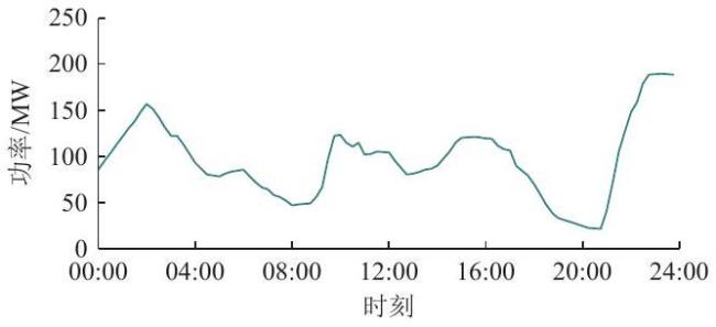
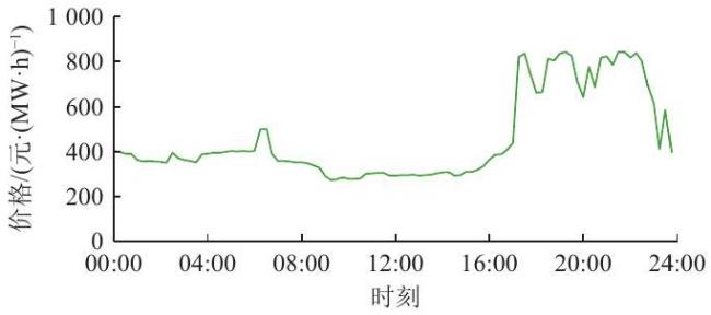
日前竞价决策时需要对次日风电发电功率和市场电价进行预测。预测的风电出力期望值曲线如图1所示  [30] ,预测误差标准差取预测出力期望值的 7%;次日电能量市场价格期望值曲线如图2所示,预测误差标准差取期望值的5%。
图1 风电出力预测期望值曲线

Fig. 1 Expected value curve of wind power output prediction

图2 日前电价预测期望值曲线

Fig. 2 Expected value curve of day-ahead electricity price prediction

场景数量的增加会导致求解效率大幅度降低,为在保证求解精度前提下具有较高的求解效率,本文对场景数的设置如下:风电出力场景生成数量取 300 个,缩减为 5 个;日前电价场景生成数量为 300 个,缩减为 20 个。由于量价曲线的功能为"根据出清电价调整申报功率",电价不确定性对量价曲线构建的影响更为直接。因此,本文设置较多的缩减后电价场景数量,以更精细地描述电价不确定性。
参考国内各省电力市场运行情况,取电能量市场曲线偏差考核价格为2倍日前电价  [30] ,量价曲线报价最大为1500元/(MW ⋅ h),最小为0元/( MW⋅h ),储能初始 SOC 为 0.5 ,末时段 SOC 为 0.5 ,SOC 上、下限分别为 0.95、0.05 。量价曲线申报段数取 5 段。

3.2 量价曲线计算结果分析

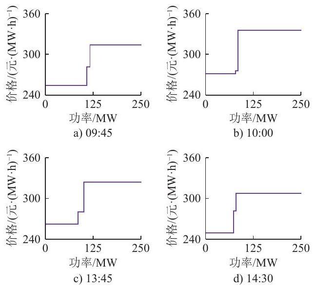
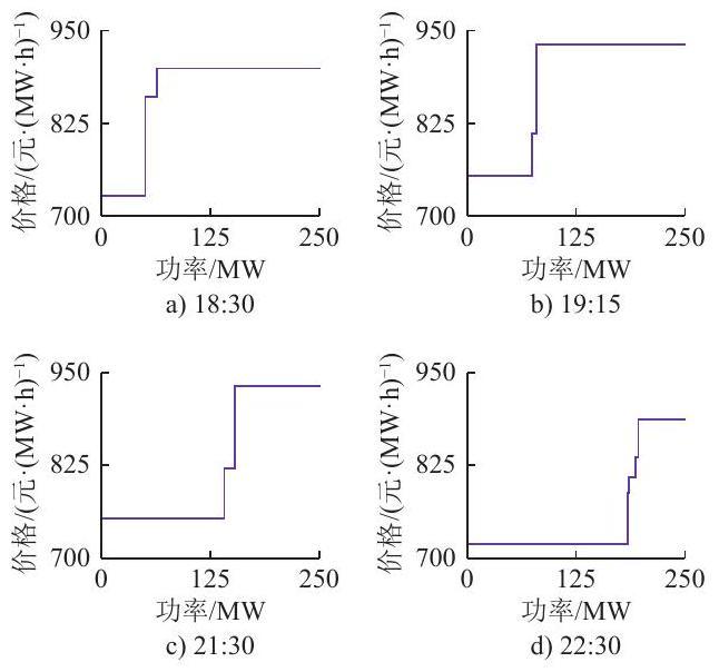
部分低、高电价时段量价曲线分别如图3图4所示;电站预期收益信息如表1所示。
图3 低电价时段量价曲线(示例时段)

Fig. 3 Price-quantity curves in low-price periods (example intervals)

为验证本文模型所生成的量价曲线在不同电价场景下为电站带来的收益表现,分别定义实际收益与理想收益作为评价指标。其中,实际收益Ip 指基于模型所得量价曲线进行申报并在特定电价场景下中标后,考虑多风电出力场景所获得的期望收益;理想收益 Iid  指在已知出清电价的条件下通过优化模型重新计算量价曲线并申报后获得的期望收益。通过计算收益偏差幅度 $\mathit{\delta }$ 评估模型性能,即
$\begin{array}{c}\mathit{\delta }=\frac{{\mathit{I}}_{\mathrm{i}\mathrm{d}}-{\mathit{I}}_{\mathrm{p}}}{{\mathit{I}}_{\mathrm{i}\mathrm{d}}}\times 100\mathit{\%}\end{array}$
图4 高电价时段量价曲线(示例时段)

Fig. 4 Price-quantity curves in high-price periods (example intervals)

表1 电站预期收益

Table 1 PPower plant expected revenue

预期收益及成本 数值
总收益/万元 105.9
日前电能量市场收益/万元 107.8
偏差考核惩罚/万元 0.7
储能寿命成本/万元 1.2
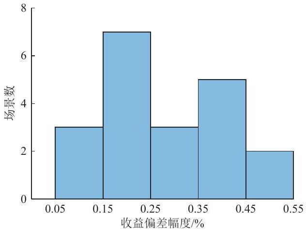
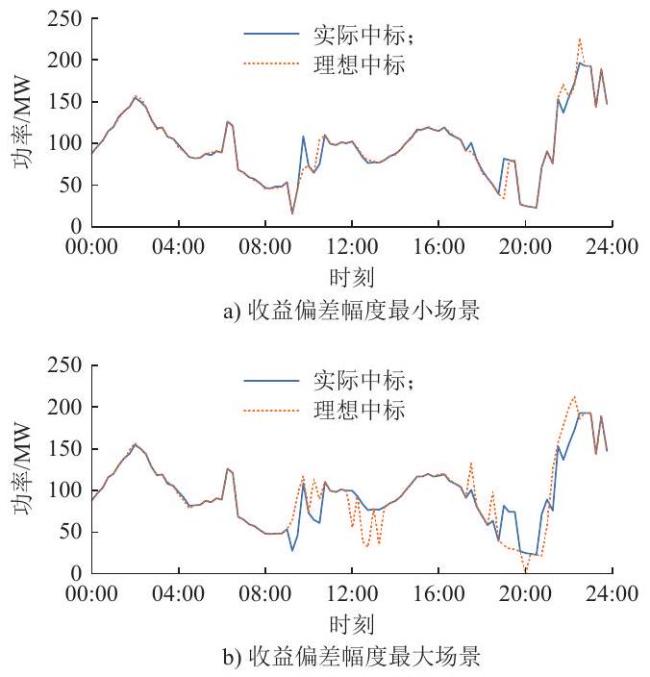
对20组电价场景分别计算了理想收益及收益偏差幅度,不同收益偏差幅度频数如图5所示。图6a)、b)分别展示了收益偏差幅度最小、最大场景下的实际中标功率与理想中标功率曲线,可以看出两者十分接近。其中,收益偏差幅度最小的场景下,电站实际收益107.26万元,与理想收益仅相差561元,收益偏差幅度为0.05%;收益偏差幅度最大的场景下,实际收益106.26万元,与理想收益相差 5830 元,收益偏差幅度为 0.55% 。
图5 收益偏差幅度频数分布

Fig. 5 Frequency distribution of revenue deviation

图6 最优与最劣收益偏差场景的实际与理想中标功率曲线

Fig. 6 Actual and ideal bid power curves under best and worst revenue deviation scenarios

结果表明,本文所构建的量价曲线决策模型能够有效适应不同电价场景,实际收益与理想收益的偏差幅度能够控制在较低水平。

3.3 报量报价方式与报量不报价方式参与市场对比分析

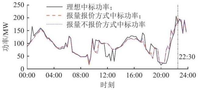
目前,部分省份的市场规则允许风储电站自行选择以报量报价方式或以报量不报价方式(作为价格接受者)参与现货市场  [34] 。本节对这两种参与市场方式进行对比分析。其中:报量报价方式下申报的量价曲线可以通过本文报价模型计算得到;报量不报价方式下申报的发电功率曲线,可以在考虑风电、电价双重不确定性的情况下,以电站期望收益最大为目标进行优化而得到。
用不确定性成本来评估报价的效果。具体而言,当实际风电出力和市场价格确定后,可以计算两种情形下的收益:基于预测数据制定的投标策略所获得的实际收益,以及在完全信息条件下(即以实际风电出力和市场价格作为已知输入)优化制定的投标策略所获得的理论最优收益。这两种收益之间的差异即为不确定性成本  [35] ,可以反映由于风电出力波动和市场电价不确定性所导致的潜在收益损失。
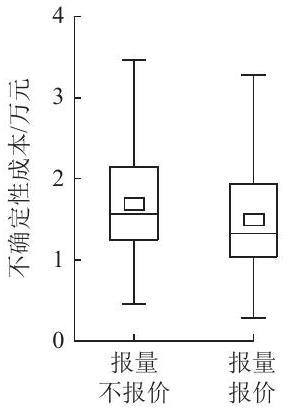
1)报量报价方式优势分析。为验证模型的有效性,通过基于自回归滑动平均模型的场景生成方法生成了600组模拟场景来模拟市场的实际运行情况以及风电出力情况。对比分析报量报价方式与报量不报价方式在各模拟场景下的不确定性成本,结果如图7所示。其中报量报价方式与报量不报价方式下的平均不确定性成本分别为1.48万元、 1.69 万元,前者相比于后者降低了约 12.4% 。这一优势主要得益于报量报价方式下量价曲线的动态调节特性,即能够根据实时电价调整中标功率,使其更接近理论最优值。相比之下,报量不报价方式在响应市场价格波动方面表现出明显的局限性。
图7 两种参与市场方式下的不确定性成本

Fig. 7 Uncertainty costs under two market participation methods

进一步对各模拟场景下两种方式的收益进行比较分析,结果如表2所示。数据分析表明,在大部分模拟场景中,报量报价方式的收益表现更为优异。这验证了所构建的报量报价模型的实用性和经济性。
表2 两种申报方式的模拟场景收益优势统计

Table 2 Statistical dominance of two bidding methods under simulation scenarios

总收益更高的申报方式 模拟场景数量 比例/%
报量报价 503 83.8
报量不报价 97 16.0
2)特殊场景下局限性分析。在少数模拟场景中,报量不报价方式的收益反而高于报量报价方式,这一现象源于量价曲线的固有特性:报量报价方式通过量价曲线动态调整中标功率来适应电价变化,通常能更好地逼近理论最优曲线。但最优中标功率实则由风电出力、出清电价和储能策略共同决定,而量价曲线仅能针对电价调整功率,故无法保证在所有场景下都达成最优。本文提出的量价曲线构建模型能够在多数情况下提高电站收益,但在部分小概率场景中,其表现反而不如报量不报价方式。
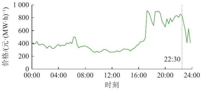
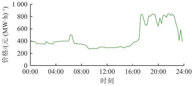
针对示例模拟场景,图8给出了该模拟场景的出清电价,图9给出了该模拟场景下的理想中标功率、作为价格接受者方式下的中标功率和报量报价方式下的中标功率。以该模拟场景中的22:30时段为例:该时段申报的量价曲线将电价高于预测期望值时的申报功率设定为高于风电预测期望值,反之则申报较低功率。在该模拟场景中,由于实际出清电价高于预测期望值,故得到了高于风电预测期望值的中标功率。然而,在该模拟场景下,该时段的实际风电出力低于预测期望值,并且由于前一小时电价更高,最优调度策略下储能已经以最大功率放电至耗尽,导致该时段最优中标功率应低于风电预测期望值。这一差异带来了较高的偏差惩罚,从而导致电站收益降低。
图8 示例模拟场景下的日前电价曲线

Fig. 8 Day-ahead electricity price curve under example simulation scenario

图9 示例模拟场景下的理想中标功率与两种报价方式下的中标功率

Fig. 9 Ideal awarded power and awarded power of two bidding methods under example simulation scenario

这一分析表明,虽然在大多数情况下报量报价方式更具优势,但在少数风电出力与电价的特殊场景下,作为价格接受者方式可能表现出更好的经济性。

3.4 偏差惩罚价格灵敏度分析

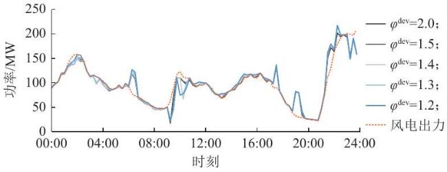
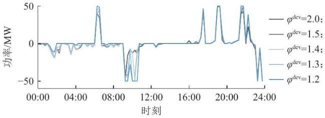
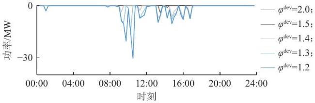
在风储电站中,储能发挥跟踪计划出力功能时获得的效益取决于偏差惩罚价格的高低;发挥"低充高放"套利功能时获得的效益取决于日前出清价差大小。决策结果会对二者相对变化产生影响。为此,本节在日前价格不变情况下,分析了不同偏差惩罚价格情境的决策结果变化情况。偏差惩罚价格取日前出清价格的 ${\mathit{\varphi }}^{\mathrm{d}\mathrm{e}\mathrm{v}}$ [30]
图10给出了某示例场景的日前电价;图11图12图13分别给出了不同偏差惩罚系数 ${\mathit{\varphi }}^{\mathrm{d}\mathrm{e}\mathrm{v}}$下,该场景中的中标功率、储能功率与偏差功率。可以看出,随着偏差惩罚系数的增加,本文报价策略在进行申报时逐渐减小套利时段申报功率与风电功率的差额。这是因为在偏差惩罚较低时,本文报价方法会用较高的储能功率容量进行套利。这一策略会带来更高的套利收益,但由于这些时段备用容量降低同样带来更多的偏差电量。而在偏差惩罚较高时,本文报价方法用更少的储能功率容量套利。这一策略会降低套利收益,但同样因增大了这些时段的备用容量而减小了偏差电量,使电站在高惩罚价格的情境中总收益更高。这表明,随着偏差惩罚价格的提高,本文模型可以通过降低储能套利功率容量来增强其跟踪计划出力的能力,进而降低偏差惩罚而提升电站整体收益。该结果同样证明了本文决策模型的有效性。
图10 示例场景下的日前电价曲线

Fig. 10 Day-ahead electricity price curve under example scenario

图11 示例场景下不同偏差惩罚系数的中标功率

Fig. 11 Awarded power under different deviation penalty coefficient under example scenario

图12 示例场景下不同偏差惩罚系数的储能功率

Fig. 12 Energy storage power under different deviation penalty coefficient under example scenario

图13 示例场景下不同偏差惩罚系数的偏差功率

Fig. 13 Deviation power under different deviation penalty coefficient under example scenario

3.5 报价段数灵敏度分析

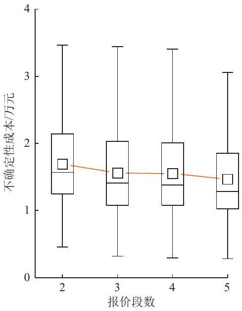
不同报价段数下的不确定性成本变化趋势如图14所示。结果表明,随着报价段数的逐步增加,不确定性成本呈现单调递减规律。这一现象的机理在于:通过增加报价段数,市场参与者能够构建更为精确的报价策略。具体而言,更为细致的分段结构使得在不同价格区间内的出力调整具备了更高的灵活性:精细化的出力意愿划分能够针对模拟场景中的价格变化实现更精准的功率调整,从而使得最终中标结果更接近于理论最优值。
图14 不同报价段数下的不确定性成本

Fig. 14 Uncertainty cost under different bidding segment numbers

4 结论

本文考虑风电出力与电价不确定性、储能寿命损耗成本及市场规则约束,构建了以各时段量价曲线的分段价格与功率长度为决策变量、以各风电-电价耦合场景下的储能充放计划为过渡变量、以最大化风储电站总期望收益为目标的随机优化决策模型。主要结论如下。
1)所提模型能够生成符合市场规则的分时段量价曲线,且所得曲线能够有效适应不同电价场景,使电站实际收益与理想收益的偏差幅度能够控制在较低水平。
2)与选择报量不报价方式参与现货市场相比,采用报量报价方式能够根据电价信号灵活调整功率申报,使中标功率更接近理论最优值,降低不确定性成本,提高整体收益。同时,增加报价段数可以提升报价策略的精细度,进一步降低不确定性成本。
3)报量报价方式并非在所有场景中都具有优势,在部分小概率场景中作为价格接受者方式的收益反而更高。这主要是因为最优中标功率由风电出力、出清电价和储能策略共同决定,而量价曲线仅能针对电价调整中标功率,在部分小概率场景下无法使中标功率达成最优。
[1]
杜刚, 赵冬梅, 刘鑫. 计及风电不确定性优化调度研究综述[J]. 中国电机工程学报, 2023, 43(7):2608-2627.

DU Gang, ZHAO Dongmei, LIU Xin. Research review on optimal scheduling considering wind power uncertainty[J]. Proceedings of the CSEE, 2023, 43(7):2608-2627.

[2]
刘英琪. 高比例风电参与的电力市场灵活运营策略研究[D]. 广州: 华南理工大学, 2020.

LIU Yingqi. Research on flexible operation strategy for high shares of wind power participating in electricity markets[D]. Guangzhou: South China University Of Technology, 2020.

[3]
国家能源局. 国家能源局关于2021年风电、光伏发电开发建设有关事项的通知[EB/OL].( 2021-05-11)[2026-04-05].

[4]
CONEJO A. NOGALES F. ARROYO J. Price-taker bidding strategy under price uncertainty[J]. IEEE Power Engineering Review, 2002, 22(9):57-63.

[5]
FAN L. WANG J. JIANG R, et al. Min-max regret bidding strategy for thermal generator considering price uncertainty[J]. IEEE Transactions on Power Systems:A Publication of the Power Engineering Society, 2014, 29(5):2169-2179.

[6]
KAZEMI M, MOHAMMADI-IVATLOO B, EHSAN M. Risk- constrained strategic bidding of gencos considering demand response[J]. IEEE Transactions on Power Systems:A Publication of the Power Engineering Society, 2015, 30(1):376-384.

[7]
SAYYAD N, KAZEM Z, MOHAMMAD R. Optimal bidding strategy of generation station in power market using information gap decision theory(IGDT)[J]. Electric Power Systems Research, 2013, 96:56-63.

[8]
SAYYAD N, KAZEM Z, MOHAMMAD A. A hybrid approach based on IGDT-MPSO method for optimal bidding strategy of price- taker generation station in day-ahead electricity market[J]. International Journal of Electrical Power and Energy Systems, 2015, 69:335-343.

[9]
SÁNCHEZ DE LA NIETA A, CONTRERAS J, MUÑOZ J. Optimal coordinated wind-hydro bidding strategies in day-ahead markets[J]. IEEE Transactions on Power Systems, 2013, 28(2):798-809.

[10]
CEREJO A, MARIANO S, CARVALHO P, et al. Hydro-wind optimal operation for joint bidding in day-ahead market:storage efficiency and impact of wind forecasting uncertainty[J]. Journal of Modern Power Systems and Clean Energy, 2020, 8(1):142-149.

[11]
王晛, 张华君, 张少华. 风电和电动汽车组成虚拟电厂参与电力市场的博亦模型[J]. 电力系统自动化, 2019, 43( 3):155-162. WANG Xian,ZHANG Huajun,ZHANG Shaohua.Game model of electricity market involving virtual power plant composed of wind power and electric vehicles[J]. Automation of Electric Power Systems,2019, 43(3):155-162.

[12]
钱韦廷, 赵长飞, 万灿, 等. 基于概率预测的混合储能平抑风电波动随机优化调控方法[J]. 电力系统自动化, 2021,45(18): 18-27. QIAN Weiting,ZHAO Changfei,WAN Can,et al. Probabilistic forecasting based stochastic optimal dispatch and control method of hybrid energy storage for smoothing wind power fluctuations[J]. Automation of Electric Power Systems,2021, 45(18):18-27.

[13]
张楠, 郭庆雷, 杜哲, 等. 面向分布式新能源聚合交易的可信合约化交易模型[J]. 中国电力, 2025, 58(9):205-218.

ZHANG Nan, GUO Qinglei, DU Zhe, et al. A trusted contract-based trading model for distributed new energy aggregation trading[J]. Electric Power, 2025, 58(9):205-218.

[14]
江婷, 王旭, 蒋传文, 等. 数据驱动下风电一抽蓄联合参与日前-实时市场随机鲁棒竞价策略[J]. 电网技术, 2022, 46(2):481-495.

JIANG Ting, WANG Xu, JIANG Chuanwen, et al. Optimal hybrid stochastic robust bidding strategy of wind and hydraulic pumped storage jointly participating in day-ahead and real-time market using data-driven method[J]. Power System Technology, 2022, 46(2): 481-495.

[15]
WANG Yuwei, ZHAO Huiru, LI Peng. Optimal offering and operating strategies for wind-storage system participating in spot electricity markets with progressive stochastic-robust hybrid optimization model series[J]. Mathematical Problems in Engineering, 2019(4):1-19.

[16]
德格吉日夫, 谭忠富, 李梦露, 等. 考虑不确定性的风储电站参与电力现货市场竞价策略[J]. 电网技术, 2019, 43(8):2799-2807.

TAN Zhongfu, LI Menglu, et al. Bidding strategy of wind-storage power plant participation in electricity spot market considering uncertainty[J]. Power System Technology, 2019, 43(8): 2799-2807.

[17]
詹隽, 黄媚, 孙晓佳, 等. 基于多时间尺度虚拟电厂鲁棒优化调节决策方法[J]. 节能, 2025, 44(11):28-33.

ZHAN Jun, HUANG Mei, SUN Xiaojia, et al. Robust optimization regulation decision-making method for virtual power plants based on multiple time scales[J]. Energy Conservation, 2025, 44(11):28-33.

[18]
杨轩, 曹晓庆, 程少靖, 等. 计及多元不确定性的虚拟电厂竞价策略[J]. 电力需求侧管理, 2025, 27(6):112-117.

YANG Xuan, CAO Xiaoqing, CHENG Shaojing, et al. Bidding strategies of virtual power plants considering diverse uncertainties[J]. Power Demand Side Management, 2025, 27(6):112-117.

[19]
KHALOIE H, ABDOLLAHI A, SHAFIE-KHAH M, et al. Coordinated wind-thermal-energy storage offering strategy in energy and spinning reserve markets using a multi-stage model[J]. Applied Energy, 2019, 259: 114168.

[20]
孙鑫, 魏文荣, 李琼林, 等. 计及不确定性的风储联合系统多时间尺度市场参与策略[J]. 电力自动化设备, 2024, 44(2):18-25.

SUN Xin, WEI Wenrong, LI Qionglin, et al. Multi-time scale market participation strategy of wind-energy storage combined system considering uncertainty[J]. Electric Power Automation Equipment, 2024, 44(2):18-25.

[21]
李咸善, 胡长宇, 张远航, 等. 风电租赁储能参与电能-调频市场竞价策略[J]. 电网技术, 2024, 48(5):1992-2002.

LI Xianshan, HU Changyu, ZHANG Yuanhang, et al. Bidding strategy of wind power rental energy storage participating infrequency regulation market[J]. Power System Technology, 2024, 48(5):1992-2002.

[22]
李钟平, 向月. 深度强化学习驱动的风储系统参与能量-调频市场竞价策略[J]. 电力工程技术, 2025, 44(3):30-42.

LI Zhongping, XIANG Yue. Deep reinforcement learning-driven bidding strategy for wind-storage systems in energy and frequency regulation markets[J]. Electric Power Engineering Technology, 2025, 44(3):30-42.

[23]
郁海彬, 董帅, 陆增洁, 等. 新型电力系统下储能参与电力调峰调频辅助市场的竞标策略[J]. 中国电力, 2023, 56(8):48-60.

YU Haibin, DONG Shuai, LU Zengjie, et al. Bidding strategy of energy storage participating in the auxiliary market of peak and frequency modulation in new power system[J]. Electric Power, 2023, 56(8):48-60.

[24]
周德群, 周显扬, 丁浩. 多市场协同下的可再生能源电力竞价策略研究[J]. 中国管理科学, 2023, 31(1):248-255.

ZHOU Dequn, ZHOU Xianyang, DING Hao. research electricity bidding on renewable strategy under multi-market coordination[J]. Chinese Journal Of Management Science, 2023, 31(1):248-255.

[25]
白庆立, 赵志鹏, 靳晓雨, 等. 考虑风电出力和电价不确定性的水风联合现货市场竞价策略[J]. 电力系统自动化, 2024, 48(11): 122-133.

BAI Qingli, ZHAO Zhipeng, JIN Xiaoyu, et al. Hydro-wind power joint bidding strategies for electricity spot market considering uncertainties of wind power output and electricity price[J]. Automation of Electric Power Systems, 2024, 48(11):122-133.

[26]
易健, 黄漪帅, 梁清鹤, 等. 现货市场下考虑预测误差的风电场日前报价策略研究[J]. 电网技术, 2025, 49(3):1079-1088.

YI Jian, HUANG Yishuai, LIANG Qinghe, et al. Research on the day ahead quotation strategy of wind farm considering prediction errors in the spot market[J]. Power System Technology, 2025, 49(3): 1079-1088.

[27]
王凯, 延肖何, 蒋凯, 等. 考虑碳交易的风光储场站参与电力现货市场报价策略与调控方法[J]. 中国电机工程学报, 2023, 43(18): 7091-7103.

WANG Kai, YAN Xiaohe, JIANG Kai, et al. Bidding strategy and regulation method for the unified wind/photovoltaic/energy storage power stations in electricity spot market considering carbon trading[J]. Proceedings of the CSEE, 2023, 43(18):7091-7103.

[28]
陆宇涛. 风光储参与现货市场的策略及技术经济研究[D]. 北京: 华北电力大学, 2024.

LU Yutao. Research on strategy and technical economy of Wind-PV-Storage Units participating in spot market[D]. Beijing: North China Electric Power Universit, 2024.

[29]
王德林, 田洪迅, 罗治强, 等. 新能源参与电力市场的实践及思考[J]. 电力系统自动化, 2025, 49(19):1-7.

WANG Delin, TIAN Hongxun, LUO Zhiqiang, et al. Practices and reflections on renewable energy participating in electricity market[J]. Automation of Electric Power Systems, 2025, 49(19):1-7.

[30]
何翔路, 娄素华, 吴耀武, 等. 双结算模式下风储一体化电站两阶段市场投标调度策略[J]. 电力系统自动化, 2022, 46(4):47-55.

HE Xianglu, LOU Suhua, WU Yaowu, et al. Two-stage market bidding and scheduling strategy of integrated wind power and energy storage station in dual-settlement mode[J]. Automation of Electric Power Systems, 2022, 46(4):47-55.

[31]
YOU Daning, LIU Hanghang, SI Juncheng, et al. Bidding strategy of wind-solar hybrid generation system in the spot market considering bidding deviation penalty[J]. IOP Conference Series:Earth and Environmental Science, 2021, 770(1):12-28.

[32]
MENG Anbo, CHEN Shun, OU Zuhong, et al. A hybrid deep learning architecture for wind power prediction based on bi-attention mechanism and crisscross optimization[J]. Energy, 2022, 238: 121795.

[33]
王荔妍, 陈启鑫, 何冠楠, 等. 考虑电池储能寿命模型的发电计划优化[J]. 电力系统自动化, 2019, 43(8):93-100.

WANG Liyan, CHEN Qixin, HE Guannan, et al. Optimization of generation scheduling considering battery energy storage life model[J]. Automation of Electric Power Systems, 2019, 43(8): 93-100.

[34]
国家能源局山东监管办公室.关于印发《山东电力市场规则(试行)》( 2026 4 月修订版)的通知[EB/OL].( 2026-05-08)[2026-05-29].

[35]
JUAN M, ANTONIO J, JUAN P. Economic valuation of reserves in power systems with high penetration of wind power[J]. IEEE Transactions on Power Systems, 2009, 24(2):900-910.

Options
Outlines

/