Study of several common instantaneous frequency calculation methods

Guang TIAN; Yan ZHAO

doi:10.6038/pg2024HH0395

Progress in Geophysics >

2024 , Vol. 39 >Issue 4: 1553 - 1564

DOI: https://doi.org/10.6038/pg2024HH0395

Study of several common instantaneous frequency calculation methods

Guang TIAN ^,¹^,² ,
Yan ZHAO ^,¹^,²^,*

Expand

¹ Key Laboratory of Exploration Technologies for Oil and Gas Resources (Yangtze University), Ministry of Education, Wuhan 430100, China
² School of Geophysics and Oil Resources, Yangtze University, Wuhan 430100, China

Received date: 2023-09-29

Online published: 2024-09-29

Copyright

Fold

Abstract

Instantaneous frequency is an important seismic attribute, which helps in identification of oil and gas reservoirs and is of great significance to reservoir prediction. This paper provides a detailed review of several common instantaneous frequency calculation methods and tests using analytical sinusoidal signals. The instantaneous frequency calculation results of each algorithm are compared with the analytical instantaneous frequency of sinusoidal signals, and various instantaneous frequency calculation methods are compared by comprehensively analyzing the correlation number, error between the calculated results and the theoretical analytical instantaneous frequency, and operation time. In order to further test the performance of each algorithm, we apply the more complex signals to each instantaneous frequency calculation method to analyze and compare. The test results of analytic and complex signals show that the performance of each algorithm varies for different types of data. The method that can relatively accurately calculate the instantaneous frequency of a simple analytical signal will have outliers, "negative frequencies", or inaccurate calculation results when calculating the instantaneous frequency of complex signals. Outliers and "negative frequencies" that appear during instantaneous frequency calculations will submerge the actual effective instantaneous frequency information. Further work is needed to overcome the problems of outliers and "negative frequencies".

Cite this article

Guang TIAN , Yan ZHAO . Study of several common instantaneous frequency calculation methods[J]. Progress in Geophysics, 2024 , 39(4) : 1553 -1564 . DOI: 10.6038/pg2024HH0395

0 引言

频率信息在地震勘探中发挥着重要作用，通过地震资料的频率信息可以得到相应的地层信息.一般情况下，人们可以通过傅里叶变换(夏竹等，2007)、时频分析(Gabor，1946；陈学华等，2008；李振春等，2010；曹思远等，2013；高静怀等，2018；刘笛等，2023)、复地震道分析(Taner et al.，1979；程乾生，1979)得到频率信息.由于波前扩散和地层衰减，地震波的频率、能量、带宽、波形是时变的(Zhao et al.，2022；Zhao, 2022, 2023；Tian et al.，2023)，是典型的非平稳信号(杨培杰等，2007；鄢高韩等，2016).傅里叶变换是一种全局变换，傅氏变换得到的是信号不同频率成分的能量分布情况，反映的是信号的全局特征，不能够反映信号某一时刻的信息(夏竹等，2007；董建华等，2007；于豪等，2013；杨培杰等，2007).因此，傅氏变换不适用于描述非平稳信号的时变频率特征(于豪等，2013).时频分析和复地震道分析中的瞬时频率则可以很好地描述非平稳信号频率的时变特征(夏竹等，2007；于豪等，2013).信号的瞬时频率反映的是信号某一时刻的频率信息，是信号某一特定时刻的局部特征.瞬时频率信息有助于确定凝析油藏和气藏，因为油气藏能够引起高频衰减(Yilmaz，2001).有学者利用瞬时频率反演地层的品质因子等参数(Matheney and Nowack, 1995；高静怀等，2008).瞬时频率对储层预测具有重要指导意义，学者们利用瞬时频率及与瞬时频率相关的信息(如甜点、甜点属性、平均瞬时频率、瞬时频率斜率等)进行河道砂体预测、指示砂岩储层、储层预测和油气检测(Radovich and Oliveros, 1998；张娥等，2000；Hart，2008；余振等，2012；尹继全和衣英杰，2013；田继先等，2016；梁岳等，2016；郑江峰等，2019；彭浩等，2022).

Gabor(1946)首次提出复信号的概念，Taner等(1979)首次将这一概念引入到地震勘探中，形成复地震道分析技术，得到三瞬参数，即瞬时振幅、瞬时频率、瞬时相位(程乾生，1979；刘财等，1995；张尔华等，2011；于捷等，2011；陈双全和李向阳，2012). 瞬时频率被广泛应用于地震勘探、声呐、雷达、医学信号等领域(Boashash，1992).瞬时频率作为地震解释中的一个重要地震属性，国内外研究人员针对瞬时频率做了大量研究工作，瞬时频率的计算得到了长足的发展(Taner et al.，1979；程乾生，1979；贺振华，1980；Scheuer and Oldenburg, 1988；Barnes, 1992, 2007；Fomel，2007；陈林和宋海斌，2009；Zhou et al.，2012；Poggiagliolmi and Vesnaver, 2014；Vesnaver，2017；张繁昌等，2016；Xing et al.，2019；Wang，2021；Liao et al.，2022).目前，针对信号的瞬时频率计算方法的准确度及计算效率的测试对比工作较少，基于此，笔者利用解析信号和复杂信号测试了多种瞬时频率计算方法.值得注意的是，笔者利用解析正弦信号对各种瞬时频率计算方法的准确度和计算效率进行了测试分析.

本文首先针对复地震道分析基本原理进行了阐述，并总结了几种瞬时频率计算方法.然后，利用简单的正弦解析信号测试各个瞬时频率计算方法，将计算结果与理论瞬时频率进行对比分析.最后，利用复杂信号对不同计算方法进行了测试和分析对比.

1 基本原理

1.1 复地震道分析

复地震道由原始地震道作为实部及其Hilbert变换得到的正交道作为虚部组成(Taner et al.，1979)，可表示为：

其中，x(t)为原始地震道；y(t)为原始地震道x(t)的Hilbert变换，即原始地震道x(t)的正交道；j为复数单位；u(t)为x(t)的复地震道.原始地震道及其正交道和复地震道的示意图如图 1所示(PetroWiki，2015).通过复地震道分析可以从原始地震道中分离出振幅信息和相位信息，得到瞬时振幅、瞬时相位和瞬时频率(Taner et al.，1979).定义复地震道的模为原始地震道的瞬时振幅(Taner et al.，1979)，记作：

显示原图|下载原图ZIP|生成PPT

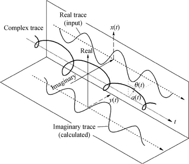
图1 复地震道示意图(PetroWiki，2015)

Fig 1 A diagram of a complex seismic trace (PetroWiki, 2015)

瞬时振幅也称为振幅包络，瞬时振幅度量的是反射强度，与某一瞬间地震信号总能量的平方根成比例.定义复地震道在某一时刻的幅角为原始地震道的瞬时相位(Taner et al.，1979)，并记作：

瞬时相位反映的是在某一时刻地震道与其虚地震道的夹角.定义原始信号瞬时相位的时间变化率为瞬时频率(Taner et al.，1979)，记作：

式中，瞬时频率f(t)的单位为Hz；ω(t)为瞬时角频率，单位为rad/s.瞬时频率其物理意义表示向量的幅角旋转速度(张贤达和保铮，1998).

原始地震道及其正交道可利用瞬时振幅和瞬时相位表示为(Taner et al.，1979)：

结合式(5)和式(6)，瞬时相位可以通过反正弦、反余弦函数进行计算(贺振华，1980)：

为了方便区分，将由式(3)、式(7)和式(8)计算得到的瞬时相位分别记作θ₁(t)、θ₂(t)、θ₃(t).

根据欧拉公式，复地震道可用极坐标表示为：

对式(9)两边同时取自然对数有：

根据式(10)可知，复地震道取自然对数后的虚部即为瞬时相位(Yilmaz，2001；Barnes，2007)，即：

其中，lm[·]表示取虚部.并将由式(11)计算得到的瞬时相位记作θ₄(t).

1.2 常见的瞬时频率估计方法

有学者认为导数运算对瞬时频率的计算有影响，所以选择利用差分运算代替导数运算(Xing et al.，2019).利用导数算子直接计算瞬时频率和利用差分计算得到的瞬时频率结果不同.因此，尽管差分和求导作用相同，但得到的计算结果不同.为此，本文针对具有相同含义计算方法的求导形式和差分形式作为两种计算方法进行分析对比.

将式(3)代入式(4)有(Taner et al.，1979)：

并将该瞬时频率计算方法简记作IFCM1(Instantaneous Frequency Calculation Method 1).

将式(7)代入式(4)有：

并将该瞬时频率计算方法简记作IFCM2.

将式(8)代入式(4)有：

并将该瞬时频率计算方法简记作IFCM3.

将式(11)代入式(4)，有：

并将该瞬时频率计算方法简记作IFCM4.

将式(3)代入式(4)，并根据求导法则进行推导可得(Taner et al.，1979)：

并将该瞬时频率计算方法简记作IFCM5，详细推导见附录A.

将式(11)代入式(4)，并进行推导可得(Yilmaz，2001；陈林和宋海斌，2009)：

并将该瞬时频率计算方法简记作IFCM6.

结合式(4)和式(11)，并利用差分表示导数运算，推导可得(陈林和宋海斌，2009)：

其中，T为时间采样间隔，并将该瞬时频率计算方法简记作IFCM7，详细推导见附录B.

用中心差分形式表达式(16)有(陈林和宋海斌，2009)：

并将该瞬时频率计算方法简记作IFCM8.

对式(16)进一步推导可得(Yilmaz，2001；Barnes，1992)，

并将该瞬时频率计算方法简记作IFCM9，详细推导见附录C.

瞬时频率是信号瞬时相位相对于时间t的一阶导数，这可能会导致瞬时频率对噪声的敏感性.根据这一观点，Zhou等(2012)为了提高瞬时频率算法的鲁棒性和稳定性，在式(16)的基础上提出了一种阻尼瞬时频率算法：

其中，e(t)=x²(t)+y²(t)，e_m=max[e(t)]，ε是阻尼因子，满足0 < ε≤1.并将该瞬时频率计算方法简记作IFCM10.

将公式(18)进一步化简可得到(Scheuer and Oldenburg, 1988；Barnes，1992)：

并将该瞬时频率计算方法简记作IFCM11，详细推导见附录D.

式(17)的离散表达式可写作(贺振华，1980)：

并将该瞬时频率计算方法简记作IFCM12，详细推导见附录E.

Poggiagliolmi和Vesnaver(2014)提出一种无需人为设置参数的瞬时频率计算方法，Wang(2021)在该算法的基础上进行改进应用，得到一种新型瞬时频率计算方法：

其中，Re[·]表示取实部，n^*(t)为n(t)的共轭，n′(t)为n(t)的时间导数，n(t)为归一化复地震道，且：

将通过式(24)这一瞬时频率计算方法简记作IFCM13.

为了方便厘清上述13种瞬时频率计算方法之间的联系，将各计算方法之间的关系绘制成图 2.

显示原图|下载原图ZIP|生成PPT

图2 各算法之间的联系缩略图

Fig 2 Thumbnail view of the relationship between the algorithms

2 简谐信号测试

利用时变频率正弦信号x(t)=sin(20πt²)测试上述13种瞬时频率计算方法.根据瞬时频率的定义，经过推导可以得到正弦信号x(t)=sin(20πt²)的理论瞬时频率f_Theory(t)=20t Hz，详细推导见附录F.图 3为该时变频率正弦信号及各计算方法的计算结果，表 1为各计算方法计算得到的瞬时频率与理论瞬时频率之间的互相关系数、均方根误差、最大绝对误差、平均绝对误差及各计算方法的运行时间.

显示原图|下载原图ZIP|生成PPT

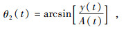
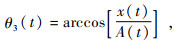
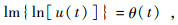
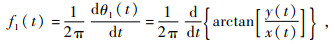
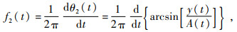
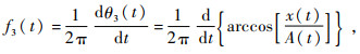
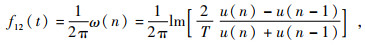
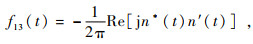
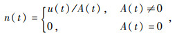
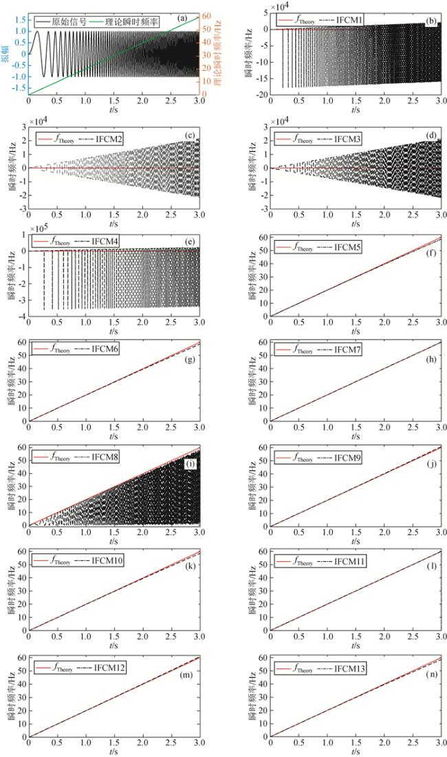
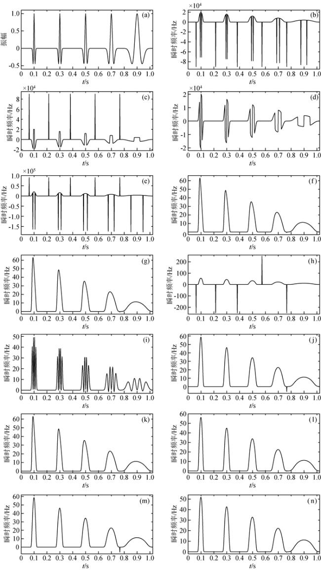
图3 时变频率正弦信号及其瞬时频率计算结果

[(a) 时变频率正弦信号及其理论瞬时频率；(b) IFCM1计算结果；(c) IFCM2计算结果；(d) IFCM3计算结果；(e) IFCM4计算结果；(f) IFCM5计算结果；(g) IFCM6计算结果；(h) IFCM7计算结果；(i) IFCM8计算结果；(j) IFCM9计算结果；(k) IFCM10计算结果；(l) IFCM11计算结果；(m) IFCM12计算结果；(n) IFCM13计算结果.

Fig 3 Time-varying frequency sinusoidal signal and its instantaneous frequency calculation results

(a) Time-varying frequency sinusoidal signal and its theoretical instantaneous frequency; (b) The result of the IFCM1 calculation; (c) The result of the IFCM2 calculation; (d) The result of the IFCM3 calculation; (e) The result of the IFCM4 calculation; (f) The result of the IFCM5 calculation; (g) The result of the IFCM6 calculation; (h) The result of the IFCM7 calculation; (i) The result of the IFCM8 calculation; (j) The result of the IFCM9 calculation; (k) The result of the IFCM10 calculation; (l) The result of the IFCM11 calculation; (m) The result of the IFCM12 calculation; (n) The result of the IFCM13 calculation.

表1 时变频率正弦信号不同瞬时频率计算方法对比

Tab 1 Comparison of different instantaneous frequency calculation methods for sinusoidal signals with time-varying frequency

	互相关系数	均方根误差	最大绝对误差	平均绝对误差	计算时长/ms
IFCM1	0.0016	42173.1802	178395.2600	19794.8015	1.6158
IFCM2	-0.0052	12100.8298	21656.4000	10376.7441	2.4933
IFCM3	-0.0009	12092.7805	21656.4000	10370.1069	1.2898
IFCM4	-0.0006	61074.7564	358036.2600	20705.1683	0.6238
IFCM5	1.0000	0.5282	1.4205	0.3469	0.6636
IFCM6	1.0000	0.5282	1.4205	0.3469	0.6594
IFCM7	1.0000	0.0100	0.0100	0.0100	0.7997
IFCM8	0.8233	21.0502	58.9493	14.9884	0.5703
IFCM9	1.0000	0.2786	0.7305	0.1895	0.5620
IFCM10	1.0000	0.5313	1.4263	0.3496	0.6982
IFCM11	1.0000	0.0100	0.0100	0.0100	0.5731
IFCM12	1.0000	0.2786	0.7305	0.1895	0.7054
IFCM13	1.0000	0.5282	1.4205	0.3469	6.1887

观察图 3发现，由对反正切、反正弦、反余弦算法得到的瞬时相位进行直接求导运算得到的瞬时频率与理论瞬时频率严重不符，计算方法IFCM1~3计算得到的瞬时频率与理论瞬时频率的互相关系数小于0.01.并且这三种方法计算得到的瞬时频率存在与实际物理意义不符的“负频率”现象.经过仔细分析，这是因为通过反正切、反正弦、反余弦算法计算得到的相位角为包裹相位(wrapped phase)(Poggiagliolmi and Vesnaver, 2014)，没有进行相位解包裹(phase unwrapping algorithm)(Poggiagliolmi and Vesnaver, 2014)，计算得到的相位值分别在

之间.致使瞬时相位在边界

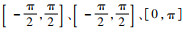
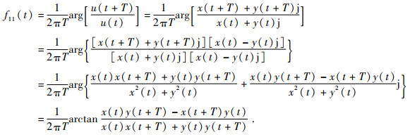
(反正切、反正弦算法求瞬时相位时)、0和π(反余弦算法求瞬时相位时)处不连续，导致瞬时相位出现骤变；当瞬时相位在不连续点处骤降时，致使在对瞬时相位进行求导时得到绝对值极大的负值；当瞬时相位在不连续点处骤增时，致使在对瞬时相位进行求导时得到绝对值极大的正值.同时计算方法IFCM1中负频率现象出现的周期较IFCM2、IFCM3计算方法更短，这是因为通过反正切、反正弦、反余弦算法计算得到的瞬时相位出现不连续点频率不同的原因.IFCM4计算得到的瞬时频率也存在“负频率”现象，这也是因为瞬时相位不连续导致瞬时相位严重跳变引起的.并且IFCM4计算得到的瞬时频率“负频率”现象更严重，其最大绝对误差较计算方法IFCM1~3要高2~16.5倍.这是因为反正切、反正弦、反余弦算法计算得到的瞬时相位骤降跨度范围为－π，而通过公式(11)计算得到的瞬时相位θ₄(t)值域为[－π, π]，瞬时相位骤降跨度范围为－2π，所以θ₄(t)骤降更严重，计算得到的负频率绝对值更大.IFCM5~13不同于IFCM1~4，IFCM1~4是通过对计算得到的瞬时相位直接进行导数运算得到的，而IFCM5~13没有对瞬时相位进行导数运算.令人高兴的是IFCM5~7、IFCM9~13计算得到的瞬时频率与理论瞬时频率一致，互相关系数约为1.0000(保留4位有效数字)，均方根误差均小于0.54，最大绝对误差均小于1.43.IFCM8的计算结果在0与理论瞬时频率之间波动，没有IFCM5~7、IFCM9~13结果好，其互相关系数为0.8233，均方根误差21.05，最大绝对误差为58.94.这是因为在利用公式(19)计算瞬时频率时，公式(19)会出现分子等于零的情况，导致IFCM8计算的瞬时频率会在理论瞬时频率与0之间波动.但值得注意的是，IFCM8没有出现“负频率”现象，相较于IFCM1~4有很大优势.同时，我们发现，IFCM5、IFCM6、IFCM8、IFCM10、IFCM13计算得到的瞬时频率略低于理论瞬时频率，IFCM9、IFCM12计算得到的瞬时频率略高于理论瞬时频率，IFCM7和IFCM11计算得到的瞬时频率与理论瞬时频率一致.

计算方法IFCM1~12的运行时长一般在0.5~2.5 ms左右，而计算方法IFCM13的运行时长达到了6.19 ms，是其他计算方法运行时长的2.4~11.0倍.这是因为计算方法IFCM13需要计算归一化后的复地震道及归一化后的复地震道的共轭和时间导数，因此其计算时间最长.

3 复杂信号测试

为了进一步探究各瞬时频率计算方法间的特点与区别，本节利用合成地震记录进行测试.为了模拟地层衰减，分别利用主频为50 Hz、40 Hz、30 Hz、20 Hz、10 Hz的雷克子波作为震源，分别在0.1 s、0.3 s、0.5 s、0.7 s、0.9 s处生成五个合成记录并叠加成一道合成地震记录，如图 4a所示，图 4b—n为各个瞬时频率计算方法的计算结果.

显示原图|下载原图ZIP|生成PPT

图4 拟地层衰减合成地震记录及其瞬时频率计算结果

(a) 合成地震记录；(b) IFCM1计算结果；(c) IFCM2计算结果；(d) IFCM3计算结果；(e) IFCM4计算结果；(f) IFCM5计算结果；(g) IFCM6计算结果；(h) IFCM7计算结果；(i) IFCM8计算结果；(j) IFCM9计算结果；(k) IFCM10计算结果；(l) IFCM11计算结果；(m) IFCM12计算结果；(n) IFCM13计算结果.

Fig 4 Simulated layer attenuation synthetic seismic record and its instantaneous frequency calculation results

(a) Synthetic seismic records; (b) The result of the IFCM1 calculation; (c) The result of the IFCM2 calculation; (d) The result of the IFCM3 calculation; (e) The result of the IFCM4 calculation; (f) The result of the IFCM5 calculation; (g) The result of the IFCM6 calculation; (h) The result of the IFCM7 calculation; (i) The result of the IFCM8 calculation; (j) The result of the IFCM9 calculation; (k) The result of the IFCM10 calculation; (l) The result of the IFCM11 calculation; (m) The result of the IFCM12 calculation; (n) The result of the IFCM13 calculation.

由图 4可知，IFCM1~4计算结果不仅存在-10⁵~-10⁴ Hz的“负频率”现象，反射界面处的瞬时频率也有近10⁴ Hz，且IFCM1~4的结果与反射界面没有表现出一致性，与其他计算方法结果差别很大，不能客观反映实际瞬时频率.IFCM5~6和IFCM9~13计算得到的瞬时频率能够很好地与反射界面一一对应，且能够反映各个反射界面处反射波频率的衰减趋势. 其中，我们注意到IFCM9和IFCM12在0.76 s附近出现了-5.9 Hz左右的“负频率”，比IFCM1~4中的负频率要低3~4个数量级.IFCM7中出现了多个-250 Hz的“负频率”，并在0.6 s处出现了一个250 Hz的瞬时频率野值，分析后认为是复地震道累积了原始地震道和正交地震道的数值突变的缘故，相较于IFCM5~6和IFCM9~13该计算方法还不够稳健.同时，值得注意的是，250 Hz也正是该数据对应的尼奎斯特频率.为了探究IFCM7中出现的±250 Hz的野值是否与数据的尼奎斯特频率有关，我们将采样时间间隔改为0.0005 s、0.001 s和0.004 s，发现利用IFCM7计算得到的瞬时频率的野值也对应变为±1000 Hz、±500 Hz和±125 Hz，即该野值与数据的尼奎斯特频率对应.其中，IFCM8结果整体上能与反射界面相对应，但其结果会出现振荡现象，没有IFCM5~7和IFCM9~13光滑，这是因为其在利用公式(19)计算瞬时频率时，公式(19)会出现分子等于零的情况，导致瞬时频率计算结果会在0与理论瞬时频率之间波动.值得注意的是，IFCM8计算的瞬时频率的负频率只有-2 Hz左右.