
Random noise suppression for pre-stack seismic data based on self-supervised learning via iterative data refinement
Received date: 2023-06-30
Online published: 2024-12-19
Copyright
The requirement of a large amount of noisy-clean training dataset is one of the main bottlenecks restricting deep learning denoising. A self-supervised pre-stack seismic random noise suppression method based on iterative data refinement is proposed, which uses only noise samples to train the deep neural networks. The method firstly uses the multiple regression theory to estimate the random noise in the common offset gathers, and then superimposes the noise components to the noisy samples to construct the strong noise samples. Taking the skip network as the model, each iteration is divided into two steps: (1) Taking the strong noise samples as input, the weak noise samples are predicted by the last iteration optimization model; (2) Constructing the nosier-noise training dataset, the network model is optimized with a supervised learning strategy. The advantages of the algorithm are as follows: (1) The noise samples that are drawn from the distribution, which is approximately the same as the actual noise, are estimated by using the characteristics of the flat events of the common offset gathers; (2) With the increase of the number of iterations, the predicted weak noise samples are similar to the actual clean samples, it is feasible to learn a self-supervised network approximating the optimal parameters of a supervised model; (3) The iterative data refinement strategy achieves data augmentation, increases the number of samples, and avoids overfitting. Experiments on synthetic and realistic noise removal demonstrate that the iterative data refinement approach achieves state-of-the-art performance.
ZhanZhan SHI , Guo HUANG , QingLi CHEN , Su PANG , YuanJun WANG . Random noise suppression for pre-stack seismic data based on self-supervised learning via iterative data refinement[J]. Progress in Geophysics, 2024 , 39(5) : 1824 -1837 . DOI: 10.6038/pg2024HH0195
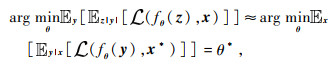
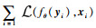 等价于求解网络参数θ的最大似然估计:
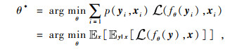
 和
和 分别为期望和条件期望,y和x分别为含噪声和纯净样本.
 和Var(x)≥Var(n),算子Var(·)表示方差,n为地震噪声)时,含噪声样本的期望近似等于纯净样本的期望
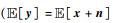
 .若对含噪声样本中混入同分布随机噪声,构造新的强噪声样本z,则其期望满足
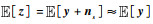 (式中ns为模拟噪声样本,并满足
 和Var[ns]≈Var[n]).假设去噪网络能够部分压制地震随机噪声,分离出随机噪声近似满足
 和Var[nd]≈Var[n](式中nd为分离出随机噪声),则去噪结果x*=x-nd满足
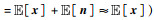
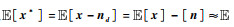 [x].利用全期望公式可以得到:
 为多元回归算法估计噪声分量.
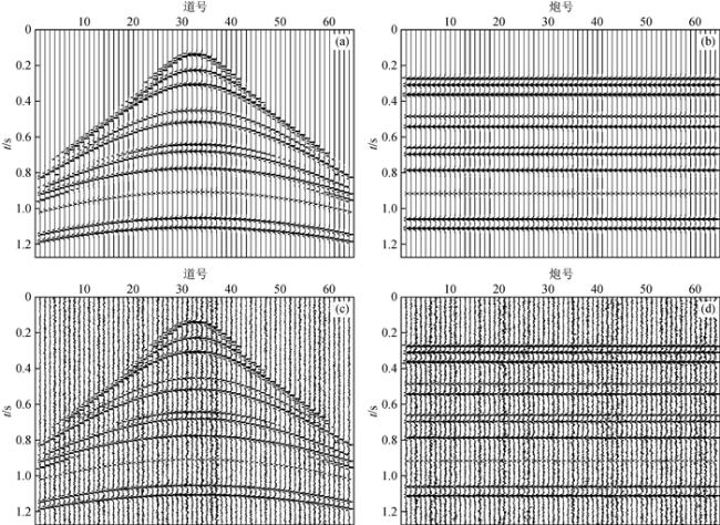
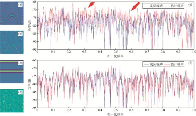
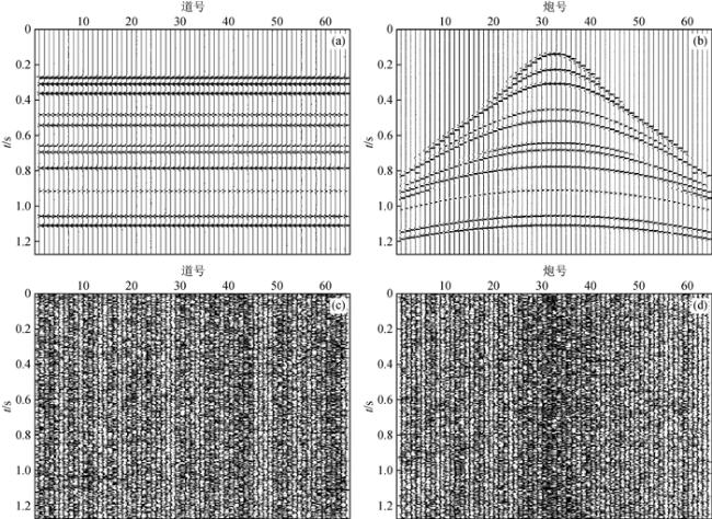
图3 2种道集估计噪声样本和噪声功率谱对比(a)共炮点道集含噪声样本;(b)多元回归算法预测样本(a)的噪声分量;(c)共炮点道集样本噪声分量(b)的功率谱; (d)共偏移距道集含噪声样本;(e)多元回归算法预测样本(d)的噪声分量;(f)共炮点道集样本噪声分量(e)的功率谱. Fig 3 Comparison of the noise samples and noise power spectrum estimated by the 2 gathers (a) Noise sample extracted from the common-shot gather; (b) Noise component of sample (a) predicted by multiple regression; (c) Power spectrum of the noise component (b); (d) Noise sample extracted from the common-offset gather; (e) Noise component of sample (b) predicted by multiple regression; (f) Power spectrum of the noise component (e). |
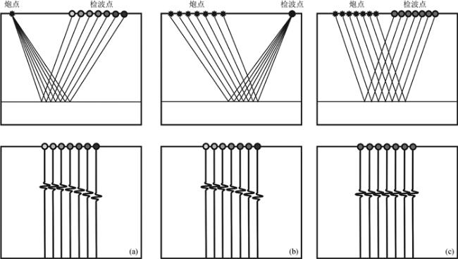
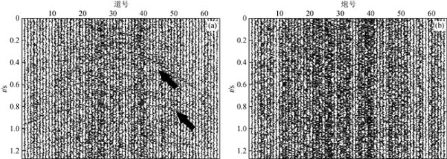
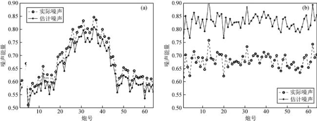
图4 2种噪声道集对比分析(a)共炮点道集;(b)共偏移距道集. Fig 4 Comparison and analysis of 2 kinds of noise gathers (a) Common-shot gather; (b) Common-offset gather. |
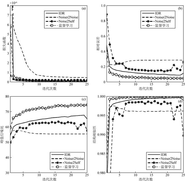
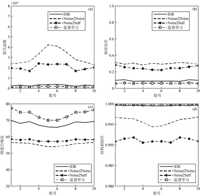
 ,其中,Pn噪声功率,Pnoisy为含噪声样本功率,实验中NdB分别取100、50和5)训练IDR算法.各组实验均采用skip网络模型,学习率为5.0e-4,批大小为64,25次迭代,利用ADAM算法优化网络模型,最小化均方根损失函数,以去噪结果的相对误差、峰值信噪比和结构相似性3种参数衡量不同模型的去噪能力.实验结果如表 1所示,可见:(1)共偏移距道集样本具有简单的纹理结构,各算法在共偏移距道集中应用效果优于共炮点道集;(2)采用估计噪声构造训练样本,IDR算法各项指标优于Noiser2Noise和Noise2Self 2种算法,性能更加接近监督学习去噪;(3)通过叠加估计噪声训练IDR算法模型,计算结果明显好于Gaussian噪声.说明了在共偏移距道集中利用多元回归理论估计噪声参与去噪模型训练能够取得较好的应用效果.
表1 去噪方法对比分析Table 1 Comparison and analysis of denoising methods |
| 道集类型 | 方法 | 噪声类型 | 损失函数 | 相对误差/% | 峰值信噪比/dB | 结构相似性 |
| *最后5个样点的平均值. | ||||||
| 共偏移距道集 | IDR | 估计噪声 | 2.98e-08 | 9.10% | 67.6 | 0.999 |
| NdB=100 | 1.92e-07 | 24.1% | 57.3 | 0.995 | ||
| NdB=50 | 4.44e-07 | 51.9% | 55.8 | 0.976 | ||
| NdB=5 | 2.04e-08 | 103% | 47.6 | 0.925 | ||
| 监督学习 | 估计噪声 | 8.21e-08 | 4.71% | 74.4 | 0.999 | |
| Noise2Self | 估计噪声 | 4.36e-07 | 19.39%* | 60.47* | 0.995* | |
| Noiser2Noise | 估计噪声 | 1.80e-07 | 13.9% | 63.4 | 0.998 | |
| 共炮点道集 | IDR | 估计噪声 | 2.54e-07 | 30.6% | 56.7 | 0.991 |
| NdB=100 | 1.49e-07 | 61.5% | 48.8 | 0.962 | ||
| NdB=50 | 2.35e-07 | 49.2% | 50.7 | 0.959 | ||
| NdB=5 | 2.16e-08 | 102% | 44.5 | 0.938 | ||
| 监督学习 | 估计噪声 | 2.81e-07 | 8.78% | 66.2 | 0.999 | |
| Noise2Self | 估计噪声 | 1.91e-06 | 33.7% | 54.7 | 0.995 | |
| Noiser2Noise | 估计噪声 | 2.37e-07 | 37.4% | 53.3 | 0.993 | |
图8 共偏移距道集IDR去噪结果和滤波残差(a)共偏移距道集去噪结果;(b)去噪结果抽取共炮点道集;(c)共偏移距道集处理残差;(d)共炮点道集残差. Fig 8 IDR denoising results and filter residuals of the common offset gathers (a) The denoising results of the common-offset gather; (b) Denoised common-shot gather is drawn from the denoising results of the common-offset gather; (c) The residual corresponding to (a); (d) The residual corresponding to (b). |
表2 不同参数配置下神经网络性能对比Table 2 Comparison of the performance of the deep neural network with different parameter configuration |
| 训练样本尺寸 | 中间变量参数量/MB | 样本数量 | 损失函数 | 相对误差/% | 峰值信噪比/dB | 结构相似性 | 训练时长/s |
| 32×32 | 1.42 | 4500 | 6.06e-08 | 12.1 | 65.8 | 0.996 | 63.1 |
| 9000 | 3.81e-08 | 12.45 | 64.74 | 0.996 | 124.95 | ||
| 18000 | 6.13e-08 | 11.80 | 66.0 | 0.999 | 345.4 | ||
| 64×64 | 5.69 | 4500 | 6.33 e-08 | 11.9 | 64.8 | 0.998 | 194.9 |
| 9000 | 3.15e-08 | 10.99 | 66.8 | 0.999 | 352.19 | ||
| 18000 | 2.98e-08 | 9.10 | 67.6 | 0.999 | 700.1 |
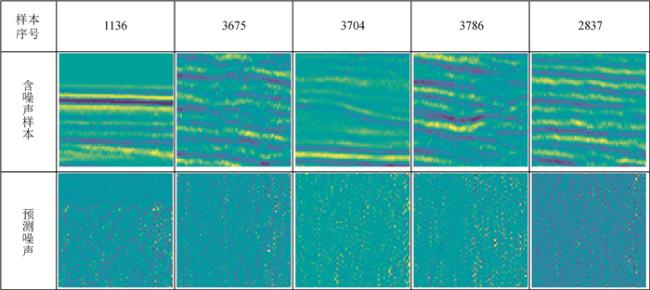
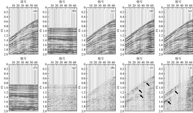
图9 共偏移距道集样本噪声估计(a)原始共炮点道集;(b)IDR去噪结果;(c)IDR去噪结果抽取共炮点道集;(d)Noise2Self去噪结果抽取共炮点道集;(e)小波变换去噪结果抽取共炮点道集;(f)原始共偏移距道集;(g)IDR滤波残差;(h)(c)对应的残差剖面;(i)Noise2Self残差剖面;(j)小波变换残差剖面. Fig 9 Noise estimation of common offset gathers |
图10 实际地震资料共偏移距道集去噪处理Fig 10 Actual seismic data denoising processing in the common-offset gathers (a) Original common-shot gather; (b) Denoising result of IDR; (c) Denoised common-shot gather is drawn from the denoising results of the common-offset gather; (d) Denoising result of Noise2Self which is performed in the common-offset gather; (e) Denoising result of wavelet transform; (f) Original common- offset gather; (g) The residual of IDR; (h) The residual corresponding to (c); (i) The residual of Noise2Self; (j) The residual of wavelet transform. |
表3 实际数据不同参数配置下损失函数对比Table 3 Comparison of loss functions under different parameter configurations for actual data |
| 样本尺寸 | 32×32 | 64×64 | ||||
| 样本数量 | 4500 | 9000 | 18000 | 4500 | 9000 | 18000 |
| 损失函数 | 1.27e-4 | 1.15e-4 | 1.06e-4 | 1.04-4 | 9.46e-05 | 6.97e-05 |
| 训练时长/s | 60.3 | 122.4 | 247.7 | 174.3 | 349.6 | 1014.8 |
感谢审稿专家提出的修改意见和编辑部的大力支持!
|
|
|
|
|
|
|
|
|
|
|
|
|
|
|
|
|
|
|
|
|
|
|
|
|
|
|
|
|
|
|
|
|
|
|
|
|
|
|
|
|
|
|
|
|
|
|
|
|
|
|
|
|
|
|
|
/
| 〈 |
|
〉 |