
Principle and Application of Algae Concentration Prediction Models in Lakes and Reservoirs
Received date: 2024-03-08
Revised date: 2024-04-03
Online published: 2024-07-01
Supported by
Key Technology Research and Development Program of Shandong(2020CXGC011406)
National Natural Science Foundation of China(22076091)
“One river, one plan, one map, one list analysis and emergency drill service of key rivers in Chengdu”(N5101012023000142-1)
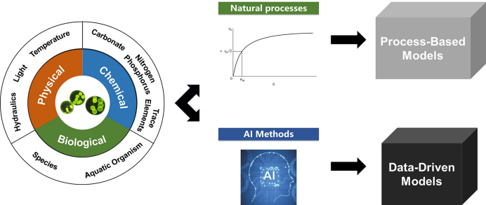
the risk of algal blooms has significantly increased in eutrophic lakes and reservoirs due To the global climate change and anthropogenic pollution,which has a significant impact on the safety and stability of municipal water supplies.to protect source water,it is necessary to construct a mathematical model and alert system to predict algae concentration in lakes and reservoirs.This paper reviews the main environmental factors(physical,chemical,and biological)that affect the algae growth,and summarizes the principles and application scenarios of existing models.Prediction models can generally be divided into two categories:process-based models(PB models)and data-driven models(DD models).PB models are based on natural processes,which enhances their interpretability and generality.However,they require a high level of research and testing,which can be costly.DD models rely on artificial intelligence methods such as machine learning,which offer flexible and diverse modeling approaches.However,they depend on data quality,lack mechanism support,and are location-specific.Both models have been extensively studied in the past decades and have been applied in some lakes and reservoirs.to further improve model performance,future research should improve the frequency and quality of data monitoring and combine natural process mechanisms with artificial intelligence methods。
1 Introduction
1.1 Eutrophication
1.2 Impacts of algal blooms
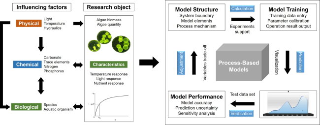
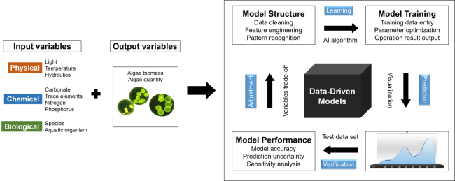
2 Influencing Factors
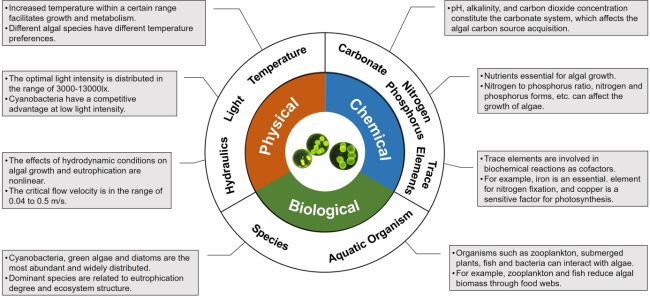
2.1 Physical factors
2.2 Chemical factors
2.3 Biological factors
3 Algae concentration prediction model
3.1 Process-based models
3.2 Data-driven models
3.3 Pro and cons
4 Conclusion and suggestions
Yuxuan Xie , Jun Wang , Yuqing Tang , Yun Zhu , Zehui Tian , Alex T. Chow , Chao Chen . Principle and Application of Algae Concentration Prediction Models in Lakes and Reservoirs[J]. Progress in Chemistry, 2024 , 36(9) : 1412 -1424 . DOI: 10.7536/PC240313
表1 Kinetic Equations for Growth and Decay of AlgaeTable 1 Kinetic equations of algae growth and decay |
| NO. | Model content | Model evaluation | Ref |
|---|---|---|---|
| 1 | Growth kinetic equation: ∂CA/∂t=(RG-RD-Q/V)·CA-Graz·Z Algae growth: RG=μmax·f(T)·f(I)·f(TN)·f(TP) ① Temperature response: f(T)=exp[-(2.3|T-Topt|)/15] ② Light response: f(I)=I/(I+KI) ③ Nutrients response: f(TN)=TN/(TN+KN); f(TP)=TP/(TP+KP) Algae decay ⑤ Cell death: RD=Mmax·e(2.3/15.0)(Topt-T)·CA/(CA+KM)·KP/(TP+KP)T≤Topt; RD=Mmax·CA/(CA+KM)·KP/(TP+KP)T>Topt ⑥ Aquatic organisms predation: Graz=Gmax·CA/(CA+KZ) | The simulation results of each sampling point in Taihu Lake showed that the model had good stability and the simulated values could fit the measured values well, but the fitting effect had not been evaluated quantitatively. The growth model parameters measured in the laboratory might differ from that in actual environment, which resulted in the error between the simulated values and measured values. | 68 |
| 2 | Growth kinetic equation: ∂CA/∂t=(RG-RD-S)·CA Algae growth: RG=μmax·f(I)·f(T)·f(NP) ① Temperature response: f(T)=1-(T-Topt)2/(Topt)2 ② Light response: f(I)=I/Iopt·exp(1-I/Iopt) ③ Nutrients response: f(NP)=min[TP/(KP+TP),TN/(KN+TN)] Algae decay: RD=R+M ④ Respiratory metabolism: R=kR·θRT-20 ⑤ Cell death: M=kM ⑦ Algae Settlement: S=vS/H | The results showed temperature and total phosphorus were the primary factors influencing algae growth in Taihu Lake. The research did not involve the fitting effect of the model to the actual data, but rather aimed to explore the main factors affecting the algae growth in Taihu Lake through the sensitivity analysis of model parameters. | 50 |
| 3 | Growth kinetic equation: ∂CA/∂t=(RG-RD-S)·CA Algae growth: RG=μmax·f(T)·f(I)·f(TN)·f(TP) ① Temperature response: f(T)=θGT-20 ② Light response: f(I)=I/(KI+I) ③ Nutrients response: f(TN)=TN/(KN+TN); f(TP)=TP/(KP+TP) Algae decay: RD=R+M ④ Respiratory metabolism: R=kR·θRT-20 ⑤ Cell death: M=kM ⑦ Algae Settlement: S=vS/H | The model's predicted value aligned well with the measured data, with an average relative error of less than 20%. This suggested that the model could accurately reflect the dynamic growth of algae to a certain extent. The model showed potential for predicting algal blooms in shallow and temperate lake systems. | 70 |
| 4 | Growth kinetic equation ∂CA/∂t={μmax·min[f(TP):f(TN):f(I)-R-M]f(T)·CA-Kraz·fraz(T)Z·fraz(CA)·CA ① Temperature response: f(T)=θR T-20 ② Light response: f(I)=(I/Iopt)·e(1-I/Iopt) ③ Nutrients response: f(TP)=(TP-TPmin)/(TPmax-TPmin); f(TN)=(TN-TNmin)/(TNmax-TNmin) ④ Respiratory metabolism: R=kR ⑤ Cell death: M=kM ⑥ Aquatic organisms predation: Graz=Kraz·fraz(T)·Zfraz(CA)·TP; fraz(CA)= CA/(KZ+ CA); fraz(T)=θrazT-20 | The one-dimensional Water quality model (DYRESM Water Quality) combined hydrodynamics and ecological process models to simulate water quality. The core equations of the ecological process components were phytoplankton growth and nutrient cycling. Simulation results for chlorophyll a indicate an average error of 24.1% and a standard deviation of 19.7% when compared to measured values. | 66,67 |
表2 Summary of model parametersTable 2 Summary of model parameters |
| Meaning | Unit | Symbol | Meaning | Unit | Symbol | |
|---|---|---|---|---|---|---|
| Algae biomass | mg/L | CA | Optimum growth temperature | ℃ | Topt | |
| Specific growth rate | d-1 | RG | Light intensity half-saturation coefficient | μE/(m2∙s) | KI | |
| Specific decay rate | d-1 | RD | Optimal light intensity | μE/(m2∙s) | Iopt | |
| Aquatic animal biomass | mg/L | Z | Total nitrogen half-saturation coefficient | mg/L | KN | |
| Predation rate | d-1 | Graz | Total phosphorus half-saturation coefficient | mg/L | KP | |
| Respiratory metabolic rate | d-1 | R | Maximum mortality | d-1 | Mmax | |
| Mortality | d-1 | M | Mortality half-saturation coefficient | mg/L | KM | |
| Settlement rate | d-1 | S | Maximum predation rate | d-1 | Gmax | |
| Water temperature | ℃ | T | Predation half-saturation coefficient | mg/L | KZ | |
| Light intensity | μE/(m2∙s) | I | Respiration rate | d-1 | kR | |
| Total nitrogen concentration | mg/L | TN | Temperature influence coefficient on respiration | 1 | θR | |
| Total phosphorus concentration | mg/L | TP | Constant mortality | d-1 | kM | |
| Lake reservoir discharge | m3/d | Q | Constant settlement rate | m/d | vS | |
| Lake reservoir area | m2 | V | Temperature influence coefficient on growth | 1 | θG | |
| Water depth | m | H | Aquatic predation rate constant | 1 | Kraz | |
| Maximum specific growth rate | d-1 | μmax | Temperature influence coefficient on predation | d-1 | θraz |
表3 Algae prediction model based on data-driven methodTable 3 Algae prediction models based on data-driven methods reported |
| Modeling method | Model content and evaluation | Ref |
|---|---|---|
| Multiple stepwise regression | · The standardized regression equation was: ln(TB+1)=1.16×ln(WT+1)+5.4×ln(TP+1)-2.33. In this equation, TB represented the total algae biomass, WT represented the water temperature, and TP represented the total phosphorus. · The correlation coefficient for the prediction model of total algae biomass was 0.65, indicating a significant correlation. · During the high algal phase in summer, the model was unable to simulate the effects of wind waves and lake currents, resulting in a significant discrepancy between the predicted and measured values. | 78 |
| Binary logistic regression model | · The log-likelihood function was: ln L(α,β)=∑ni=1[yi(α+β’Xi)-ln(1+eα+β’Xi)] · The model's predicted probability closely matched the outbreak frequency between April and October, but was slightly lower during January to March and November to December. The trends remained consistent. · The model was imprecise when the lake was heterogeneous and not well-mixed, and it neglected information on the intensity of the bloom outbreak. | 81 |
| Generalized additive Models (GAMs) | · Construct generalized additive models to determine the nutrient standard. Use chlorophyll a as the response variable and total nitrogen, total phosphorus and monthly average surface air temperature as the explanatory variables. · The model parameters were found to be significant (p < 0.001), and the AIC and GCV results indicated appropriate explanatory variables. · The results indicated that an increase in water temperature would significantly decrease the nutrient standard values. It was recommended to strictly control the total phosphorus to suppress algal blooms. | 82 |
| Autoregressive Integrated Moving Average Model (ARIMA) | · An autoregressive integrated moving average (ARIMA) model was established for the daily concentration of chlorophyll a, and compared with a multivariate linear regression (MVLR) model. · The MVLR model required several inputs, while the ARIMA model only required one input variable. However, the ARIMA model might not provide a clear understanding of the mechanisms that affect algal blooms. · The Index of Agreement (IoA) for the ARIMA model was 0.86, significantly higher than that of the MVLR model (0.55), indicating greater potential for early warning applications. | 84 |
| Wavelet analysis combined with artificial neural network (ANN) | · A single-parameter wavelet neural network (WNN) approach was constructed to predict harmful algal blooms (HAB). The approach demonstrated high accuracy in predicting HAB in both a lake and a reservoir. · Compared to ARIMA and ANN models, the WNN model performed better with an R value of up to 0.986 and an average absolute error as low as 0.103×10⁴ cells/mL. · Reliable and precise forecasts required daily data on cell density or chl a, which might be impractical for some applications due to limited budgets. | 85 |
| Hybrid Evolutionary Algorithm (HEA) | · Inferential models using the hybrid evolutionary algorithm (HEA) were developed to achieve a 10- to 30-day-ahead prediction on concentrations of cyanobacteria cells or cyanotoxins. · Model performance R2 ranged from 0.3 to 0.7 depending on the output index (cells or microcystins), study site, prediction time and validation methods. | 86 |
表4 Comparison of Process Mechanism Model and Data Driven ModelTable 4 Comparison between process-based models and data-driven models |
| Process-Based models | Data-Driven models | |
|---|---|---|
| Advantage | 1. Good interpretability and generalization ability. 2. Identify the bloom triggers and assist in decision and management. | 1. The model performs better on specific problems. 2. Do not rely on professional knowledge 3. Modeling methods are diverse and flexible. |
| Disadvantage | 1. Many unknown parameters require experimental calibration. 2. The mechanisms behind part of the processes are still unclear. 3. Huge modeling cost and high application threshold. | 1. Lack interpretability and generalization and have the risks of falling into local optimality and overfitting. 2. Usually only applicable to specific data and regions. 3. The model structure and parameters need to be adjusted according to the system status changes. |
| Similarity | 1. Rely on monitoring data. Models cannot be built without sample data. 2. The appropriate method should be selected according to the modeling conditions and objectives. 3. There is a general trend to combine knowledge of process mechanisms with data mining and analysis methods. | |
| [1] |
|
| [2] |
|
| [3] |
|
| [4] |
|
| [5] |
|
| [6] |
|
| [7] |
|
| [8] |
|
| [9] |
|
| [10] |
|
| [11] |
|
| [12] |
|
| [13] |
|
| [14] |
|
| [15] |
|
| [16] |
|
| [17] |
|
| [18] |
|
| [19] |
|
| [20] |
|
| [21] |
|
| [22] |
|
| [23] |
|
| [24] |
|
| [25] |
|
| [26] |
|
| [27] |
(张悦. 城市供水系统应急净水技术指导手册. 第2版. 北京: 中国建筑工业出版社, 2017.).
|
| [28] |
|
| [29] |
|
| [30] |
|
| [31] |
|
| [32] |
|
| [33] |
|
| [34] |
(刘雪梅, 章光新. 水科学进展, 2022, 33(02): 316.)
|
| [35] |
|
| [36] |
|
| [37] |
|
| [38] |
(龚川, 贡丹丹, 刘德富, 张佳磊, 严广寒. 环境科学研究, 2020, 33(05): 1214.).
|
| [39] |
|
| [40] |
(秦伯强, 王小冬, 汤祥明, 冯胜, 张运林. 地球科学进展, 2007, 22(9): 896.).
|
| [41] |
|
| [42] |
|
| [43] |
|
| [44] |
(梁培瑜, 王烜, 马芳冰. 湖泊科学, 2013, 25(04): 455.).
|
| [45] |
|
| [46] |
|
| [47] |
|
| [48] |
|
| [49] |
|
| [50] |
|
| [51] |
|
| [52] |
|
| [53] |
|
| [54] |
|
| [55] |
|
| [56] |
|
| [57] |
|
| [58] |
(孔繁翔, 马荣华, 高俊峰, 吴晓东. 湖泊科学, 2009, 21(3): 314.).
|
| [59] |
|
| [60] |
|
| [61] |
|
| [62] |
|
| [63] |
|
| [64] |
|
| [65] |
|
| [66] |
|
| [67] |
|
| [68] |
(许秋瑾, 秦伯强, 陈伟民, 陈宇炜, 高光. 湖泊科学, 2001, (02): 149.).
|
| [69] |
|
| [70] |
|
| [71] |
|
| [72] |
|
| [73] |
|
| [74] |
|
| [75] |
|
| [76] |
|
| [77] |
|
| [78] |
(陈宇炜, 秦伯强, 高锡云. 湖泊科学, 2001, (01): 63.).
|
| [79] |
|
| [80] |
|
| [81] |
|
| [82] |
|
| [83] |
|
| [84] |
|
| [85] |
|
| [86] |
|
| [87] |
|
| [88] |
|
| [89] |
|
| [90] |
|
| [91] |
|
| [92] |
|
| [93] |
|
| [94] |
|
| [95] |
(王小艺, 赵载平, 刘载文, 许继平, 董硕琦. 环境科学学报, 2012, 32(07): 1677.).
|
/
| 〈 |
|
〉 |