
Anti-interference processing for CSAMT based on deep learning and joint de-noising
Received date: 2023-09-03
Online published: 2024-09-29
Copyright
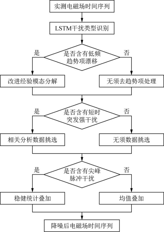
Controlled-Source Audio Magnetotelluric (CSAMT) is a near-surface geophysical method that developed on the basis of Magnetotelluric method (MT). With the development of social economy,the data quality of CSAMT has also been seriously disturbed by noise interference. In practical exploration,the time series of electromagnetic field is usually superimposed with large-scale trend drift,short-term sudden strong interference and peak impulsive outliers,resulting in the distortion of the calculated resistivity spectrum. In this paper,an anti-interference processing method based on deep learning and joint de-noising is proposed to preprocess CSAMT time series. Firstly,a forward algorithm of electromagnetic time series of layered earth controllable source is proposed,which is used to generate standard electromagnetic signals without noise interference. Then,a Long and Short Term Memory Neural Network (LSTM) classifier is trained to recognize the noise. Finally,the improved Empirical Mode Decomposition (EMD) algorithm,correlation based data selection algorithm and robust statistical algorithm are jointly used to de-noise the CSAMT time series. The test results by simulated data show that the recognition accuracy of LSTM for noise interference can reach more than 95%,and the three noise reduction algorithms can reduce the data error from about 20% to less than 3%. Finally,the proposed method is applied to the actual data set of a metal mining area in Inner Mongolia. the accuracy of low-frequency resistivity and phase was effectively improved.
WeiQiang LIU , PinRong LIN , RuJun CHEN , Kun ZHANG , ChangXin CHEN , Xu LIU . Anti-interference processing for CSAMT based on deep learning and joint de-noising[J]. Progress in Geophysics, 2024 , 39(4) : 1457 -1473 . DOI: 10.6038/pg2024HH0341
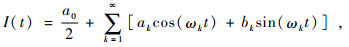
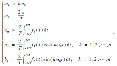

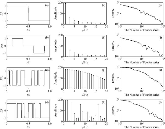
图1 人工源电磁勘探常用激励电流波形和频谱及拟合误差随傅里叶级数数量的变化曲线从上至下分别为方波、双极性波、扩频波、伪随机波等. Fig 1 Excitation current waveform and its frequency spectrum commonly used in artificial source electromagnetic exploration, the changing of waveform reconstruction error with the increase of the number of Fourier series is also shown From top to bottom are square wave, bipolar wave, spread spectrum wave, pseudo-random wave, etc. |

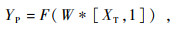
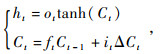
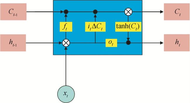
图2 一个LSTM节点的结构,当前时间步的传输单元ht, Ct受当前输入xt和前一时间步长传输单元ht-1, Ct-1的综合影响(a)原始电场和拟合电场;(b)原始磁场和拟合磁场;(c)含噪电场和拟合电场;(d)含噪磁场和拟合磁场. Fig 2 The structure of an LSTM node, the transmission units ht and Ct of the current time step is affected by the current input xt and the transmission units ht and Ct of the previous time step |
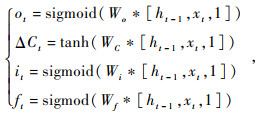
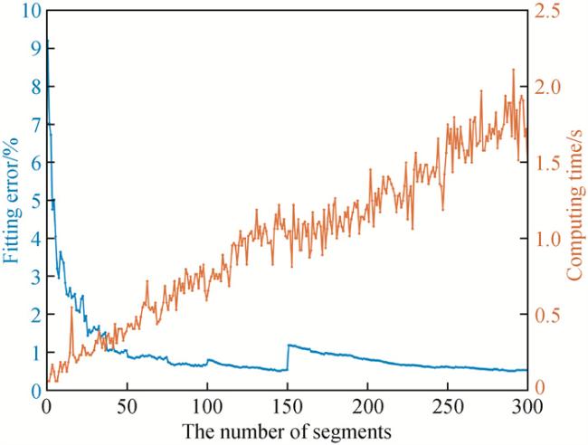
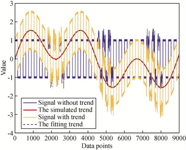
图4 在改进的经验模态分解算法中,拟合误差和时间成本随参数n的变化Fig 4 Variation of fitting error and time cost with parameter n in the modified empirical mode decomposition algorithm |
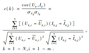

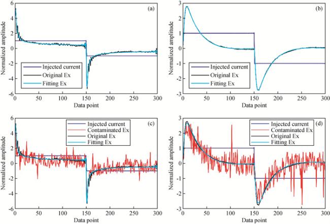
图6 原始电磁场和波形拟合电磁场对比示意图Fig 6 Comparison diagram of original electromagnetic field and fitting electromagnetic field (a) Original electric field and fitting electric field; (b) Original magnetic field and fitting magnetic field; (c) Noisy electric field and fitting electric field; (d) Noisy magnetic field and fitting magnetic field. |
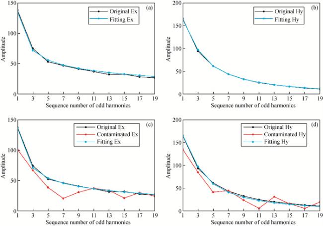
图7 原始电磁场、受污染电磁场和拟合电磁场的低频频谱(只有前19个奇谐波)(a)原磁场和拟合磁场的频谱;(b)原磁场和拟合磁场的频谱;(c)原磁场、污染磁场和拟合磁场的频谱;(d)原磁场、污染磁场和拟合磁场的频谱. Fig 7 The low-frequency spectrum (only the first 19 odd harmonics) of the original, contaminated, and fitting electromagnetic fields (a) The spectrums of original and fitting electric fields; (b) The spectrums of original and fitting magnetic fields; (c) The spectrums of original, contaminated and fitting electric fields; (d) The spectrums of original, contaminated and fitting magnetic fields. |
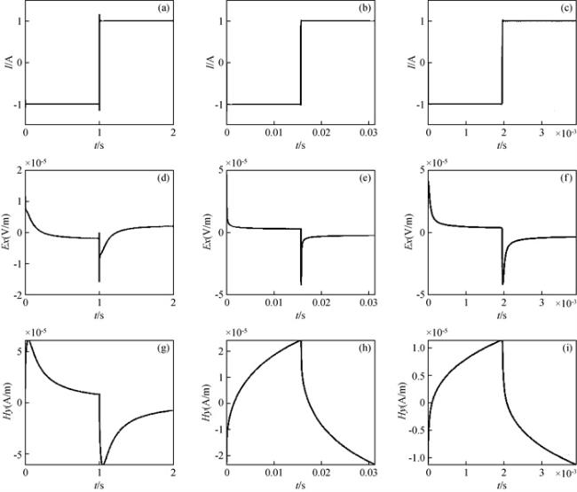
图8 三个高质量电磁场的时间序列(a)、(b)和(c)分别是基频0.5 Hz、32 Hz和256 Hz的发射电流;(d)、(e)和(f)分别是基频0.5 Hz、32 Hz和256 Hz的电场;(g)、(h)和(i)分别是基频0.5 Hz、32 Hz和256 Hz的磁场. Fig 8 Time series of three high-quality electromagnetic fields (a), (b) and (c) are emission currents with fundamental frequencies of 0.5 Hz, 32 Hz and 256 Hz, respectively; (d), (e) and (f) are electric fields with fundamental frequencies of 0.5 Hz, 32 Hz and 256 Hz, respectively; (g), (h) and (I) are magnetic fields with fundamental frequencies of 0.5 Hz, 32 Hz and 256 Hz, respectively. |
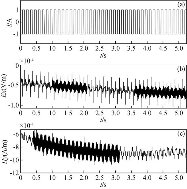
图9 对两层大地模型正演的电磁场添加噪声干扰后的波形(基频为32 Hz)(a)发射电流;(b)感应电场;(c)感应磁场. Fig 9 Waveform after adding noise interference to the electromagnetic field forward simulated by the two-layer geodetic model (the fundamental frequency is 32 Hz) (a) Emission current; (b) Induced electric field; (c) Induced magnetic field. |
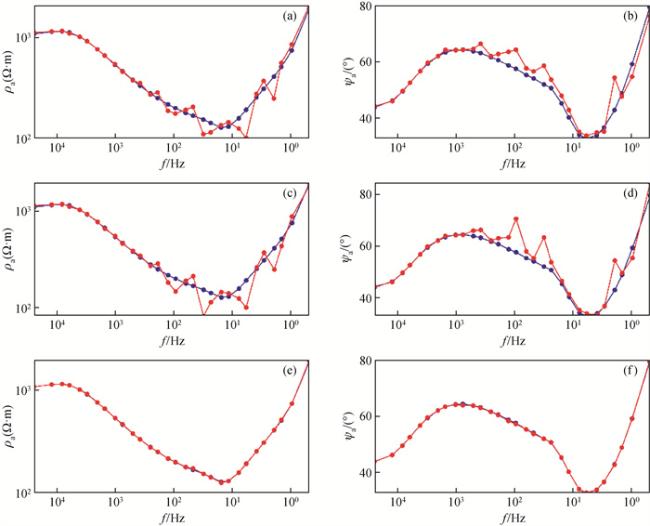
图10 通过三种方法得到的视电阻率和视相位,并与真实值作对比(a)和(b)为均值叠加法获得的视电阻率和相位;(c)和(d)为稳健叠加法获得的视电阻率和相位;(e)和(f)为联合降噪法获得的视电阻率和相位. Fig 10 Apparent resistivity and apparent phase obtained by three methods and compared with the real values (a) and (b) are the apparent resistivity and phase obtained by the mean superposition method; (c) and (d) are the apparent resistivity and phase obtained by the robust superposition method; (e) and (f) are the apparent resistivity and phase obtained by the joint noise reduction method. |
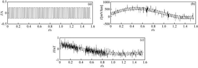
图11 加入仿真噪声的电磁场数据(基频为32 Hz)(a)激励电流;(b)加入仿真噪声干扰的电场;(c)加入仿真噪声干扰的磁场. Fig 11 Electromagnetic field data with simulated noise (fundamental frequency is 32 Hz) (a) Excitation current; (b) Electric field with simulated interferences; (c) Magnetic field with simulated noise interference. |
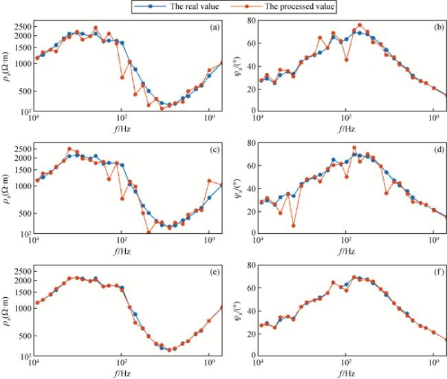
图12 通过三种方法得到的视电阻率和视相位,并与真实值作对比(a)和(b)为均值叠加法获得的视电阻率和相位;(c)和(d)为稳健叠加法获得的视电阻率和相位;(e)和(f)为联合降噪法获得的视电阻率和相位. Fig 12 Apparent resistivity and apparent phase obtained by three methods and compared with the real values (a) and (b) are the apparent resistivity and phase obtained by the mean superposition method; (c) and (d) are the apparent resistivity and phase obtained by the robust superposition method; (e) and (f) are the apparent resistivity and phase obtained by the joint noise reduction method. |
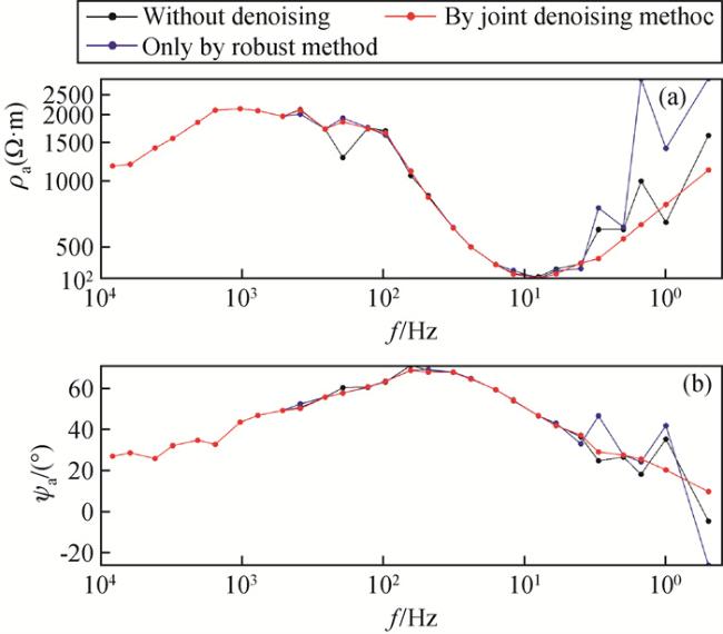
图13 采用三种方法对某测点实测电磁场数据进行处理所得视电阻率和视相位曲线黑线为常规多次叠加方法,蓝线为稳健叠加方法,红线为本文联合降噪方法. Fig 13 Apparent resistivity and apparent phase curves obtained by processing the measured electromagnetic field data of a measuring point with three methods The black line is the conventional multiple superposition method, the blue line is the robust superposition method, and the red line is the joint noise reduction method. |
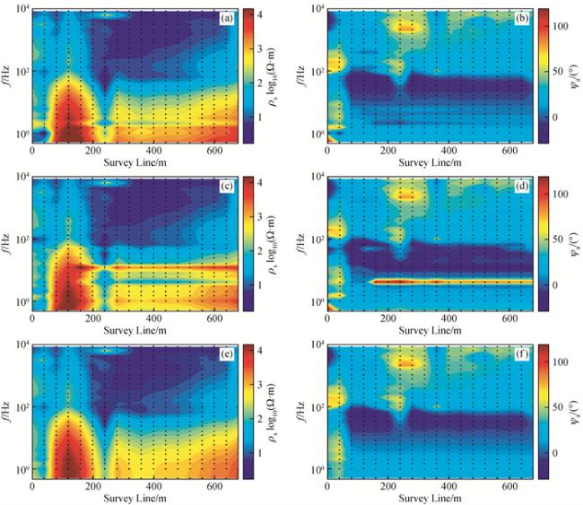
图14 采用三种方法对电磁场时间序列进行处理后计算得到某测线视电阻率和视相位拟断面图(a)和(b)为常规多次叠加方法;(c)和(d)为稳健叠加方法;(e)和(f)为联合降噪方法. Fig 14 The apparent resistivity and apparent phase pseudo profiles of a survey line are calculated after processing the electromagnetic field time series with three methods (a) and (b) are conventional multiple stacking methods; (c) and (d) are robust stacking methods; (e) and (f) are joint noise reduction methods. |
感谢中南大学、长沙巨杉科技公司等单位对本研究的帮助,感谢审稿专家对本文提出的修改意见.
|
|
|
|
|
|
|
|
|
|
|
|
|
|
|
|
|
|
|
|
|
|
|
|
|
|
|
|
|
|
|
|
|
|
|
|
|
|
|
|
|
|
|
|
|
|
|
|
|
|
|
|
|
|
|
|
|
|
|
|
|
|
|
|
|
|
|
|
|
|
|
|
|
|
|
|
|
|
|
|
|
|
|
|
|
|
|
|
|
|
|
|
|
|
|
|
|
|
|
|
|
|
|
|
|
|
|
|
|
|
|
|
|
|
/
| 〈 |
|
〉 |