
Bayesian inversion: an important method and challenge for seismic source parameter inversion research
Received date: 2023-10-17
Online published: 2024-12-19
Copyright
The role of geophysical inversion in seismic research and prediction is of paramount importance. This paper seeks to comprehensively outline the constraints associated with conventional inversion techniques, focusing on the introduction of a Bayesian-based uncertainty inversion method. Bayesian inversion involves computing posterior distributions utilizing diverse prior distributions and likelihood functions, with special emphasis on established techniques like the Markov Chain Monte Carlo (MCMC) and variational inference methods, thereby augmenting the reliability of inversion outcomes.The manuscript furnishes an elaborate exposition on pivotal techniques within Bayesian inversion, notably delving into regularization methods (such as Laplace and von Karman regularization) that confine the parameter space in seismic inversion, validated through rigorous case studies. Moreover, it expounds on sampling methodologies (including the Metropolis-Hastings algorithm and Gibbs sampling) that facilitate parameter space sampling and approximate posterior distributions. The application of the Metropolis-Hastings algorithm in seismic inversion is meticulously elucidated.The discussion accentuates the criticality of model parameter selection, notably the influence of uncertainty associated with fault geometric shape selection on inversion results. Additionally, it probes into the challenges encountered in constructing finite fault source models and presents a Bayesian-based case study evaluating the credibility of different slip model clusters.In conclusion, the paper summarizes the limitations inherent in the Bayesian approach and delineates potential avenues for future research directions. In the realm of geophysical inversion, the application of Bayesian methods presents novel prospects for overcoming the constraints of traditional methodologies.
Zhe WANG , YunHua LIU . Bayesian inversion: an important method and challenge for seismic source parameter inversion research[J]. Progress in Geophysics, 2024 , 39(5) : 1771 -1787 . DOI: 10.6038/pg2024HH0340
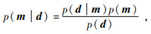
 ,观测误差服从正态分布,那么高斯似然函数可以表示为(Bagnardi and Hooper, 2018):
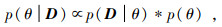
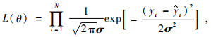 ,观测误差服从Poisson分布,那么Poisson似然函数可以表示为(赵志文等,2008):
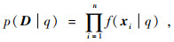
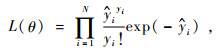 ,那么残差平方和似然函数可以表示为(彭军还,1994):
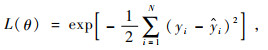
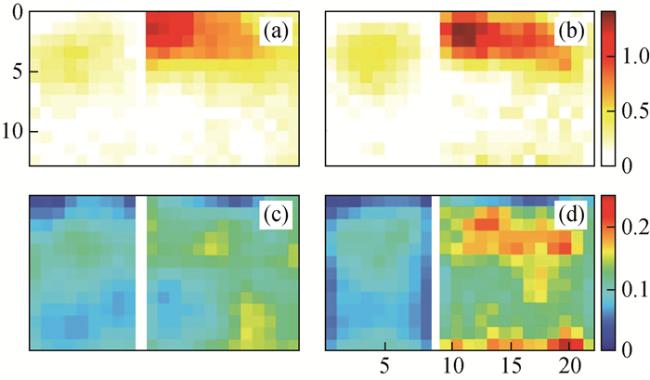
图2 (a) 采用冯卡门先验和(b)拉普拉斯先验的贝叶斯反演的断层滑动分析(众数);(c,d)是对应的断层滑动分布标准偏差(修改自Amey et al., 2018)两种方法反演的滑动分布大致相似,但最大滑动量位置有所不同,因为拉普拉斯在沿着走向方向上延伸了断层的滑动(如右图所示),并且在断层东北段上施加了更大的滑动.从标准偏差可以看出,拉普拉斯先验正则化的不确定性更明显. Fig 2 The Bayesian inversion of fault slip using (a) von Mises and (b) Laplace priors (modes); (c, d) Corresponding standard deviation of the fault slip distribution (adapted from Amey et al., 2018) The slip distributions retrieved by both methods are approximately similar, yet the location of maximum slip differs as Laplace extends slip along the strike direction of the fault (as shown in the right panel) and applies greater slip on the northeast fault. From the standard deviation, it is evident that the Laplace prior regularization exhibits more pronounced uncertainty. |
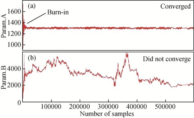
图3 (a) 收敛的马尔可夫链和(b)未收敛的马尔可夫链的示例追踪图(修改自Bagnardi and Hooper, 2018)前20000次迭代也被丢弃作为调整最大步长的燃烧期的一部分,因为变化的步长可能导致对后验概率密度函数的非典型抽样. Fig 3 (a) Example trace plot of a converged Markov chain and (b) example trace plot of a non-converged Markov chain (modified from Bagnardi and Hooper, 2018) The first 20000 iterations were also discarded as part of the burn-in period for adjusting the maximum step length, as variable step lengths can lead to non-typical sampling of the posterior probability density function. |
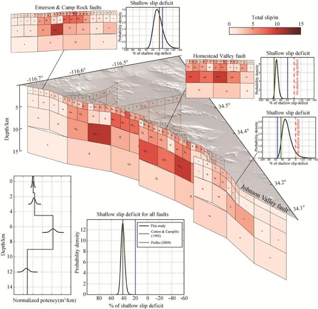
图4 后续平均余震滑动模型(修改自Gombert et al., 2018)每个子断层补丁的颜色表示滑动幅度.箭头及其相关的95%置信度椭圆表示滑动方向和不确定性.左下角的插图显示了按深度分的规范化破裂能.整个断层系统和各个断层段的浅滑动缺陷(SSD)的概率密度函数(PDF)被呈现.同一图上的垂直线表示两个已发表模型(Cotton and Campillo, 1995; Fialko,2004)的SSD. Fig 4 Shows the time-averaged postseismic sliding model (modified from Gombert et al., 2018) The color of each subfault patch represents the magnitude of sliding. Arrows and their associated 95% confidence ellipses represent the direction of sliding and its uncertainty. The inset in the bottom left corner displays the normalized rupture energy distribution as a function of depth. The Probability Density Functions (PDFs) of Shallow Slip Deficit (SSD) for the entire fault system and individual fault segments are presented. Vertical lines on the same figure represent the SSDs of two published models (Cotton and Campillo, 1995; Fialko, 2004). |
感谢审稿专家提出的修改意见和编辑部的大力支持!
|
|
|
|
|
|
|
|
|
|
|
|
|
|
|
|
|
|
|
|
|
|
|
|
|
|
|
|
|
|
|
|
|
|
|
|
|
|
|
|
|
|
|
|
|
|
|
|
|
|
|
|
|
|
|
|
|
|
|
|
|
|
|
|
|
|
|
|
|
|
|
|
|
|
|
|
|
|
|
|
|
|
|
|
|
|
|
|
|
|
|
|
|
|
|
|
|
|
|
|
|
|
|
|
|
|
|
|
|
|
|
|
|
|
|
|
|
|
|
|
|
|
|
|
|
|
|
|
|
|
|
|
|
|
|
|
|
|
|
|
|
|
|
|
|
|
|
|
|
|
|
|
|
|
|
|
|
|
|
|
|
|
|
|
|
|
|
|
|
|
|
|
|
|
|
|
|
|
|
|
|
|
|
|
|
|
|
|
|
|
|
|
|
|
|
|
|
|
|
|
|
|
|
|
|
|
|
|
|
|
|
|
|
|
|
|
|
|
|
|
|
|
|
|
|
|
|
|
|
|
|
|
|
|
|
|
|
|
|
|
|
|
|
|
|
|
|
|
/
| 〈 |
|
〉 |