
Research on two-dimensional reservoir grain size distribution prediction based on the fusion of automatic hyperparameter optimization framework and gradient boosting algorithm
Received date: 2023-08-15
Online published: 2024-12-19
Copyright
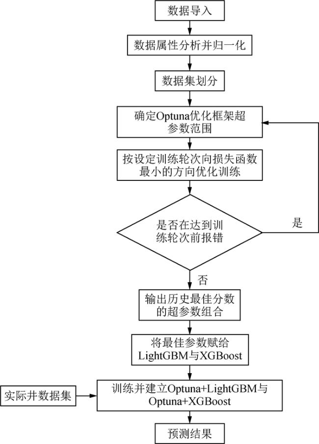
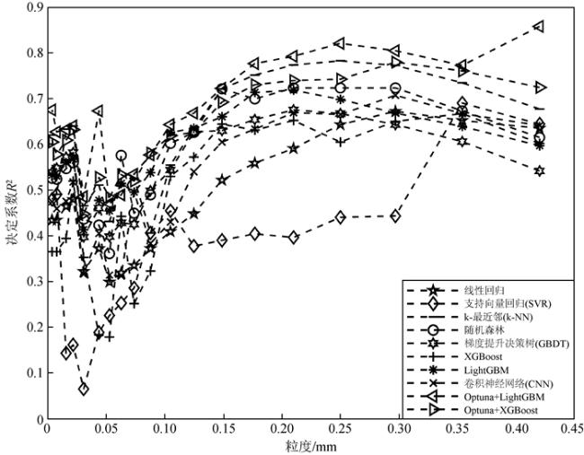
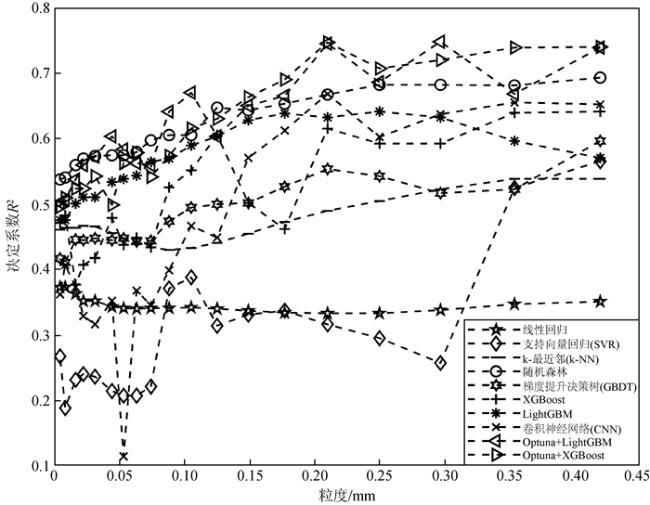
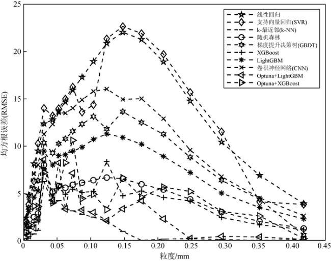
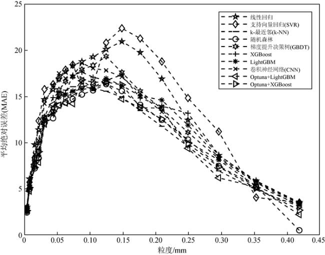
Rock grain size plays a significant role in the analysis of hydraulic conditions and the identification of depositional environments. Traditional methods for grain size measurement, for instance sieve analysis and laser diffraction, are time-consuming, costly, and suffer from discontinuity in depth due to limited core recovery during drilling. Although the combination of well log curves and machine learning methods can compensate for the limitations of rock physics experimental techniques, existing studies mainly focus on one-dimensional characteristic values of grain size, lacking a comprehensive representation of the two-dimensional grain size distribution. In this study, we propose a machine learning approach that combines the automatic hyperparameter optimization framework (Optuna) with gradient boosting algorithms (LightGBM and XGBoost) to address the challenge of predicting two-dimensional grain size distribution in reservoirs. Based on well log data and grain size distribution experimental data from a certain block in the Chengdao oilfield, we compare eight different machine learning methods, including linear regression, Support Vector Regression (SVR), k-Nearest Neighbors (k-NN), random forest, Gradient Boosting Decision Tree (GBDT), XGBoost, LightGBM, and Convolutional Neural Network (CNN). By optimizing the machine learning parameters, we identify the most appropriate method for predicting reservoir grain size distribution. The research results demonstrate significant differences in the accuracy of grain size distribution prediction among the ten machine learning methods. When using nine well log parameters, including natural potential, sonic, wellbore diameter, compensated neutron, natural gamma, formation resistivity, deep lateral resistivity, micro lateral resistivity, and shallow lateral resistivity, as inputs, the proposed method achieves the highest accuracy in predicting the two-dimensional grain size distribution in reservoirs, with R2 coefficients approaching 0.7 and smaller errors. Furthermore, linear regression, SVR, as well as GBDT attain lower accuracy in predicting reservoir grain size distribution, which are not eligible for grain size prediction in reservoirs.
Key words: Grain size distribution; Machine learning; Optuna; XGBoost; LightGBM
XiMei JIANG , WeiChao YAN , HuiLin XING , JianMeng SUN . Research on two-dimensional reservoir grain size distribution prediction based on the fusion of automatic hyperparameter optimization framework and gradient boosting algorithm[J]. Progress in Geophysics, 2024 , 39(5) : 1886 -1900 . DOI: 10.6038/pg2024HH0199


 ,以损失函数的负梯度作为当前决策树的残差近似值,不断进行迭代,使得模型的损失函数L最小化,优化的目标函数可表示为(Chen and Guestrin, 2016):

表1 历史最佳分数及超参数组合Table 1 Historical best score and hyperparameter combination |
| 超参数 | R0.420 | R0.297 | R0.210 | R0.149 | R0.105 | R0.053 | R0.016 | R0.004 |
| 目标函数历史最佳分数(值) | 0.0123 | 0.0158 | 0.0196 | 0.0283 | 0.0243 | 0.0293 | 0.0241 | 0.0278 |
| n_estimators | 436 | 176 | 195 | 229 | 366 | 247 | 325 | 397 |
| reg_alpha | 0.0723 | 0.0019 | 0.0243 | 0.0689 | 0.0101 | 0.0023 | 0.0062 | 0.0026 |
| reg_lambda | 0.2513 | 0.5598 | 0.1713 | 1.1811 | 0.0012 | 0.0118 | 1.3641 | 0.0029 |
| colsample_bytree | 0.3 | 0.7 | 1.0 | 0.9 | 0.8 | 0.4 | 0.9 | 0.9 |
| subsample | 0.6 | 0.8 | 0.6 | 0.5 | 0.8 | 0.5 | 0.7 | 0.6 |
| learning_rate | 0.0433 | 0.4882 | 0.0156 | 0.0790 | 0.1624 | 0.1110 | 0.0290 | 0.0547 |
| max_depth | 48 | 20 | 38 | 20 | 46 | 27 | 26 | 36 |
| num_leaves | 554 | 486 | 198 | 364 | 523 | 738 | 413 | 321 |
| min_child_samples | 5 | 71 | 1 | 10 | 17 | 13 | 19 | 20 |
| cat_smooth | 67 | 36 | 16 | 19 | 57 | 100 | 70 | 22 |
表2 测井曲线统计表Table 2 Logging curve statistics table |
| 曲线名称 | AC /(μm/s) | CAL /cm | CNL /% | DEN/ (g/cm3) | GR/ API | RD/ (Ω·m) | RMLL /(Ω·m) | RS /(Ω·m) | RT /(Ω·m) | SP /mV |
| 测井值 | 122.27 | 10.46 | 33.17 | 2.13 | 70.88 | 5.43 | 4.04 | 5.59 | 5.43 | 34.78 |
| 122.04 | 10.46 | 33.64 | 2.13 | 70.22 | 5.54 | 4.07 | 5.73 | 5.54 | 35.47 | |
| 124.14 | 10.46 | 32.47 | 2.13 | 71.86 | 6.02 | 3.61 | 6.27 | 6.02 | 37.02 | |
| | | | | | | | | | | |
| 100.01 | 10.69 | 35.66 | 2.38 | 101.38 | 3.61 | 4.31 | 3.49 | 3.61 | 43.93 | |
| 99.49 | 10.66 | 34.22 | 2.39 | 102.03 | 3.68 | 4.44 | 3.52 | 3.68 | 42.38 | |
| 总计个数 | 355 | 355 | 355 | 355 | 355 | 355 | 355 | 355 | 355 | 355 |
| 均值 | 120.63 | 10.37 | 34.93 | 2.14 | 82.92 | 15.22 | 4.13 | 15.1 | 11.74 | 58.8 |
| 方差 | 8.16 | 0.79 | 2.65 | 0.08 | 13.78 | 12.22 | 0.73 | 12.35 | 13.13 | 13.08 |
| 最小值 | 95.64 | 8.4 | 26.3 | 1.97 | 62.75 | 2.72 | 1.98 | 2.75 | 1.58 | 33.1 |
| 上四分位 | 115.93 | 9.66 | 33.43 | 2.08 | 71.43 | 7.25 | 3.83 | 7.07 | 4.6 | 48.38 |
| 二四分位 | 121.24 | 10.69 | 34.43 | 2.11 | 80.63 | 15.21 | 4.13 | 15.12 | 7.28 | 60.39 |
| 下四分位 | 125.19 | 10.71 | 36.06 | 2.18 | 93.46 | 15.22 | 4.30 | 15.12 | 11.36 | 68.39 |
| 最大值 | 151.03 | 14.48 | 47.34 | 2.39 | 119.52 | 64.91 | 7.88 | 66.03 | 64.91 | 85.79 |
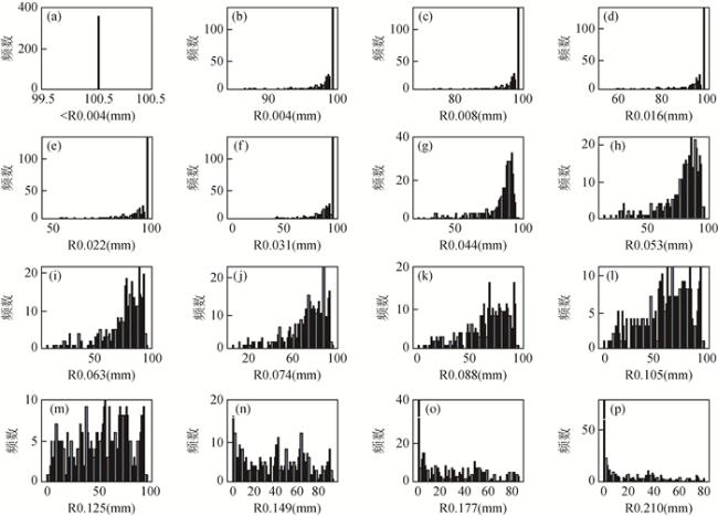
图2 粒度数据属性分布图(a)—(p)分别为粒度<0.004 mm、0.004 mm、0.008 mm、0.016 mm、0.022 mm、0.031 mm、0.044 mm、0.053 mm、0.063 mm、0.074 mm、0.088 mm、0.105 mm、0.125 mm、0.149 mm、0.177 mm、0.210 mm的数据属性分布. Figure 2 Grain data attribute distribution plot (a)—(p) Data attribute distributions with grain sizes of < 0.004 mm, 0.004 mm, 0.008 mm, 0.016 mm, 0.022 mm, 0.031 mm, 0.044 mm, 0.053 mm, 0.063 mm, 0.074 mm, 0.088 mm, 0.105 mm, 0.125 mm, 0.149 mm, 0.177 mm, 0.210 mm, respectively. |
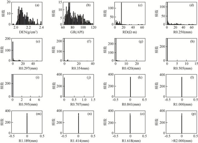
图3 粒度及部分测井数据属性分布图(a)—(c)分别为密度、自然伽马、深侧向电阻率测井曲线的数据属性分布;(d)—(p)分别为粒度0.250 mm、0.297 mm、0.354 mm、0.420 mm、0.505 mm、0.595 mm、0.707 mm、0.841 mm、1.000 mm、1.189 mm、1.414 mm、1.618 mm、≥2.000 mm的数据属性分布. Fig 3 Grain size and partial logging data attribute distribution diagram (a)—(c) Data attribute distributions of density, natural gamma and deep lateral resistivity logging curves, respectively; (d)—(p) Data attribute distributions with grain sizes of 0.250 mm, 0.297 mm, 0.354 mm, 0.420 mm, 0.505 mm, 0.595 mm, 0.707 mm, 0.841 mm, 1.000 mm, 1.189 mm, 1.414 mm, 1.618 mm, and ≥2.000 mm, respectively. |


表3 埕岛油田某区块整口井测井曲线统计表Table 3 Statistical table of logging curve of the whole well in a certain block of Chengdao oilfield |
| 曲线名称 | AC /(μm/s) | CAL /cm | CNL /% | GR /API | RD /(Ω·m) | RMLL /(Ω·m) | RS /(Ω·m) | RT /(Ω·m) | SP /mV |
| 测井值 | 88.22 | 10.66 | 56.19 | 42.66 | 0.62 | 21.54 | 0.12 | 0.62 | -63.11 |
| 88.32 | 10.65 | 55.88 | 42.60 | 0.62 | 21.59 | 0.12 | 0.62 | -63.08 | |
| 88.42 | 10.65 | 55.57 | 42.53 | 0.62 | 21.63 | 0.12 | 0.62 | -63.05 | |
| | | | | | | | | | |
| 129.87 | 10.45 | 46.24 | 86.53 | 3.16 | 2.63 | 2.57 | 2.63 | 24.12 | |
| 129.81 | 10.45 | 46.13 | 86.64 | 3.16 | 2.63 | 2.58 | 2.63 | 24.13 | |
| | | | | | | | | | |
| 109.68 | 10.30 | 37.10 | 112.66 | 3.31 | 3.28 | 3.62 | 3.31 | 51.79 | |
| 109.61 | 10.30 | 36.99 | 112.79 | 3.30 | 3.28 | 3.62 | 3.31 | 51.81 | |
| 109.55 | 10.30 | 36.88 | 112.91 | 3.30 | 3.29 | 3.63 | 3.30 | 51.84 | |
| 总计个数 | 90001 | 90001 | 90001 | 90001 | 90001 | 90001 | 90001 | 90001 | 90001 |
| 均值 | 124.45 | 11.17 | 39.20 | 89.67 | 4.47 | 3.02 | 4.05 | 4.47 | 36.53 |
| 方差 | 12.84 | 1.09 | 6.05 | 15.07 | 4.69 | 1.45 | 4.75 | 4.69 | 13.47 |
| 最小值 | 79.50 | 10.17 | 23.80 | 38.15 | 0.45 | 1.43 | 0.12 | 0.45 | -63.11 |
| 上四分位 | 114.93 | 10.48 | 34.58 | 80.98 | 3.01 | 2.34 | 2.58 | 3.01 | 28.40 |
| 二四分位 | 123.53 | 10.71 | 38.14 | 90.00 | 3.59 | 2.82 | 3.16 | 3.59 | 32.88 |
| 下四分位 | 133.30 | 11.51 | 43.44 | 99.12 | 4.57 | 3.42 | 4.11 | 4.57 | 41.94 |
| 最大值 | 173.53 | 16.83 | 68.75 | 156.12 | 65.38 | 37.16 | 66.45 | 65.38 | 84.05 |
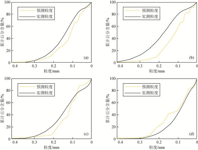
图9 粒度累计概率分布曲线Fig 9 Granularity cumulative probability distribution curve (a) Cumulative probability distribution of grain size at 1280.23 m; (b) Cumulative probability distribution of grain size at 1281.35 m; (c) Cumulative probability distribution of grain size at 1455.42 m; (d) Cumulative probability distribution of grain size at 1452.9 m. |
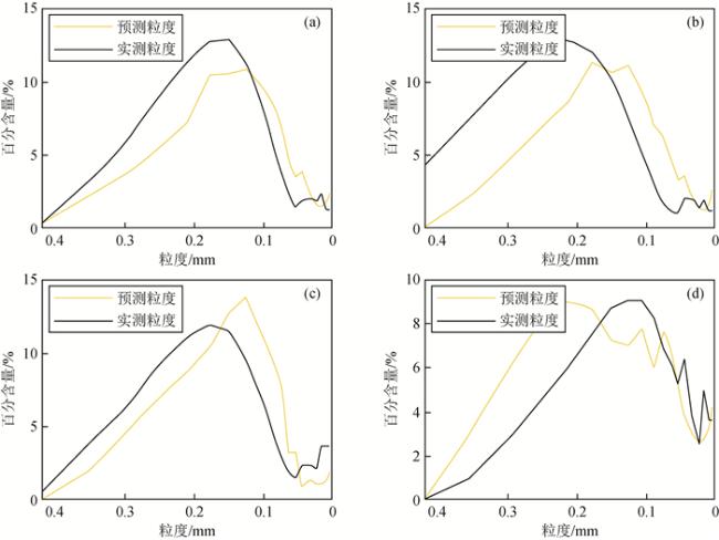
图10 粒度频率分布谱(a)1280.23 m处的粒度频率分布;(b)1281.35 m处的粒度频率分布;(c)1455.42 m处的粒度频率分布;(d)1452.9 m处的粒度频率分布. Fig 10 Grain size frequency distribution spectrum (a) Frequency distribution of grain size at 1280.23 m; (b) Frequency distribution of grain size at 1281.35 m; (c) Frequency distribution of grain size at 1455.42 m; (d) Frequency distribution of grain size at 1452.9 m. |
表4 四个深度点粒度实测数据与预测数据的粒度评估参数Table 4 Granularity evaluation parameters for measured and predicted data at four depth points |
| 预测数据 | |||||||
| 深度/m | 中值粒径/mm | 平均粒径/mm | 峰度 | 分选系数 | 标准离差 | 偏差 | |
| 1280.23 | 0.125 | 0.1263 | 0.5968 | 0.3559 | -0.07816 | -0.0114 | |
| 1281.35 | 0.105 | 0.1487 | 0.9096 | 0.3559 | -0.09992 | -0.2164 | |
| 1455.42 | 0.105 | 0.115 | 0.4536 | 0.4181 | -0.05789 | -0.1112 | |
| 1452.9 | 0.088 | 0.1097 | 0.5916 | 0.2994 | -0.08202 | -0.1258 | |
| 实测数据 | |||||||
| 1280.23 | 0.125 | 0.1327 | 0.6769 | 0.4971 | -0.07932 | -0.0566 | |
| 1281.35 | 0.177 | 0.1873 | 0.5907 | 0.4200 | -0.10346 | -0.0701 | |
| 1455.42 | 0.125 | 0.122 | 0.5394 | 0.3523 | -0.08914 | 0.02022 | |
| 1452.9 | 0.088 | 0.0957 | 0.6049 | 0.2953 | -0.07602 | -0.04908 | |
感谢审稿专家提出的修改意见和编辑部的大力支持!
|
|
|
|
|
|
|
|
|
|
|
|
|
|
|
|
|
|
|
|
|
|
|
|
|
|
|
|
|
|
|
|
|
|
|
|
|
|
|
|
|
|
|
|
|
|
|
|
|
|
|
|
|
|
|
|
|
|
|
|
|
|
|
|
|
|
|
|
|
|
|
|
|
|
|
|
|
|
|
|
|
|
|
|
|
|
|
|
|
|
/
| 〈 |
|
〉 |