
Feasibility analysis of constructing a regional gravitational model using the method of spherical harmonics analysis
Received date: 2024-03-29
Online published: 2025-03-13
Copyright
Technical methods related to the regional gravity fields, include precise geoid determination, downward continuation of gravity anomalies, and construction of regional models, which are greatly faced with challenges, such as low accuracy or efficiency, computation approximations, instability, and lack of criterion. This study introduces the fast implementation technique of ultra-high degree spherical harmonics analysis into the construction of regional gravity field, combined with satellite gravity field models of low to medium frequency spectrum and GNSS/leveling data. By employing a 5400-degree spherical harmonics analysis (SHA), it is possible to achieve a regional gravity field reconstruction with a resolution of 2 arc-minutes and an error less than 1 mGal for gravity anomalies, less than 1 cm for (quasi) geoid, and less than 0.4 arc-seconds for vertical deflection. Meanwhile, SHA can also be used for stable downward continuation of airborne gravity anomalies, which is verified to be more simple, accurate, and stable. Therefore, SHA is worth promoting and applying in the modeling of regional gravity fields and related data processing problems.
XinXing LI , JinKai FENG , HaoPeng FAN , XiaoGang LIU , Diao FAN , ShanShan LI . Feasibility analysis of constructing a regional gravitational model using the method of spherical harmonics analysis[J]. Progress in Geophysics, 2025 , 40(1) : 11 -24 . DOI: 10.6038/pg2025II0047
表1 计算环境参数Table 1 Computing environment parameters |
| 计算环境 | 参数 |
|---|---|
| 操作系统 | Windows10 64bit |
| CPU | Intel(R) Core(TM) i7-9750H CPU @ 2.60 GHz |
| 内存/GB | 32 |
| 线程数 | 1 |
| 软件环境 | VS 2019/C++/Eigen/Intel MKL |
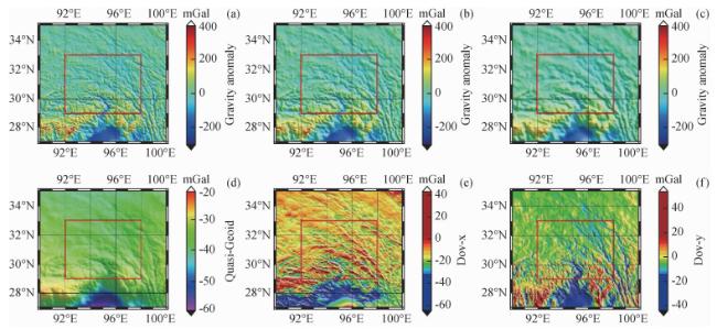
图5 局部重力场各场元仿真结果(a)地面重力异常;(b)3000 m重力异常;(c)8000 m重力异常;(d)地面高程异常;(e)地面垂线偏差子午分量;(f)地面垂线偏差卯酉分量. Fig 5 The simulation results of various field elements of the local gravitational field (a) Ground gravity anomaly; (b) 3000 m gravity anomaly; (c) 8000 m gravity anomaly; (d) Abnormal ground elevation; (e) Ground vertical deviation meridian component; (f) The vertical deviation of the ground is the Maoyou component. |
表2 Model1模型重建局部重力场误差统计表Table 2 Error statistics of the reconstructed local gravity field using Model1 |
| 统计量/单位 | 数据量 | Max | Min | Mean | Std | Rms |
|---|---|---|---|---|---|---|
| Δg1-Δg0(0 m)/mGal | 240×300 | 19.217 | -19.731 | -0.090 | 0.567 | 0.575 |
| Δgair1-Δgair(3000 m)/mGal | 240×300 | 58.108 | -63.672 | -0.012 | 2.419 | 2.419 |
| Δgair1-Δgair(8000 m)/mGal | 240×300 | 72.672 | -62.945 | 0.105 | 3.690 | 3.692 |
| ζ1-ζ0/m | 240×300 | 53.832 | 34.768 | 41.580 | 2.630 | 41.663 |
| ξ1-ξ0/arc sec(″) | 240×300 | 56.610 | -10.017 | 1.141 | 4.056 | 4.214 |
| η1-η0/arc sec(″) | 240×300 | 22.902 | -3.795 | 5.350 | 1.370 | 5.523 |
图6 Model1模型重建局部重力场误差分布图(a)地面重力异常;(b)3000 m重力异常;(c)8000 m重力异常;(d)地面高程异常;(e)地面垂线偏差子午分量;(f)地面垂线偏差卯酉分量. Fig 6 Distribution of reconstructed local gravity field errors using Model1 (a) Ground gravity anomaly; (b) 3000 m gravity anomaly; (c) 8000 m gravity anomaly; (d) Abnormal ground elevation; (e) Ground vertical deviation meridian component; (f) The vertical deviation of the ground is the Maoyou component. |
表3 Model1模型重建局部重力场扣除边界区域后的误差统计表Table 3 Error statistics of the reconstructed local gravity field using Model1 after deducting a certain boundary |
| 统计量 | 扣除边界大小 | 数据量 | Max | Min | Mean | Std | Rms |
|---|---|---|---|---|---|---|---|
| Δg1-Δg0(0 m)/mGal | 0.5° | 210×270 | 2.869 | -2.916 | -0.090 | 0.258 | 0.273 |
| 1.0° | 180×240 | 1.503 | -1.906 | -0.089 | 0.232 | 0.248 | |
| 2.0° | 120×180 | 0.781 | -1.020 | -0.089 | 0.204 | 0.223 | |
| Δgair1-Δgair(3000 m)/mGal | 0.5° | 210×270 | 1.389 | -1.117 | -0.041 | 0.170 | 0.175 |
| 1.0° | 180×240 | 0.411 | -0.349 | -0.045 | 0.077 | 0.089 | |
| 2.0° | 120×180 | 0.066 | -0.163 | -0.048 | 0.030 | 0.057 | |
| Δgair1-Δgair(8000 m)/mGal | 0.5° | 210×270 | 1.137 | -2.346 | -0.022 | 0.266 | 0.267 |
| 1.0° | 180×240 | 1.137 | -0.549 | 0.030 | 0.199 | 0.202 | |
| 2.0° | 120×180 | 0.252 | -0.159 | 0.021 | 0.068 | 0.071 | |
| ζ1-ζ0/m | 0.5° | 210×270 | 48.705 | 36.554 | 41.464 | 2.027 | 41.514 |
| 1.0° | 180×240 | 46.479 | 37.532 | 41.379 | 1.599 | 41.410 | |
| 2.0° | 120×180 | 43.859 | 38.925 | 41.275 | 0.987 | 41.286 | |
| ξ1-ξ0/arc sec(″) | 0.5° | 210×270 | 11.010 | -3.964 | 0.757 | 2.527 | 2.638 |
| 1.0° | 180×240 | 6.894 | -2.829 | 0.643 | 1.976 | 2.078 | |
| 2.0° | 120×180 | 3.697 | -1.682 | 0.559 | 1.218 | 1.340 | |
| η1-η0/arc sec(″) | 0.5° | 210×270 | 11.496 | 1.619 | 5.375 | 1.080 | 5.482 |
| 1.0° | 180×240 | 9.390 | 3.154 | 5.356 | 0.885 | 5.428 | |
| 2.0° | 120×180 | 6.722 | 3.858 | 5.307 | 0.610 | 5.342 |
表4 Model2、Model3模型重建局部重力场误差统计表Table 4 Error statistics of the reconstructed local gravity field using Model2 and Model3 |
| 统计量 | 扣除边界大小 | 数据量 | Max | Min | Mean | Std | Rms |
|---|---|---|---|---|---|---|---|
| Δg236-Δg0(0 m)/mGal | 0° | 240×300 | 18.405 | -18.864 | -0.022 | 0.543 | 0.543 |
| 2.0° | 120×180 | 0.885 | -0.945 | -0.021 | 0.203 | 0.205 | |
| Δg3300-Δg0(0 m)/mGal | 0° | 240×300 | 11.439 | -12.522 | -0.001 | 0.463 | 0.463 |
| 2.0° | 120×180 | 0.872 | -0.945 | -0.001 | 0.200 | 0.200 | |
| ζ236-ζ0/m | 0° | 240×300 | 8.396 | -2.463 | 1.030 | 1.178 | 1.564 |
| 2.0° | 120×180 | 2.038 | 0.281 | 0.986 | 0.418 | 1.070 | |
| ζ3300-ζ0/m | 0° | 240×300 | 1.166 | -0.664 | 0.064 | 0.066 | 0.092 |
| 2.0° | 120×180 | 0.103 | 0.013 | 0.056 | 0.014 | 0.058 | |
| ξ236-ξ0/arc sec(″) | 0° | 240×300 | 48.253 | -9.891 | 1.111 | 2.468 | 2.706 |
| 2.0° | 120×180 | 1.606 | -0.019 | 0.492 | 0.266 | 0.559 | |
| ξ3300-ξ0/arc sec(″) | 0° | 240×300 | 12.323 | -16.475 | -0.008 | 0.523 | 0.523 |
| 2.0° | 120×180 | 0.159 | -0.150 | 0.003 | 0.034 | 0.035 | |
| η236-η0/arc sec(″) | 0° | 240×300 | 19.116 | -6.782 | 0.368 | 1.506 | 1.551 |
| 2.0° | 120×180 | 1.793 | -1.367 | 0.090 | 0.559 | 0.566 | |
| η3300-η0/arc sec(″) | 0° | 240×300 | 7.516 | -7.600 | 0.005 | 0.323 | 0.323 |
| 2.0° | 120×180 | 0.235 | -0.142 | 0.010 | 0.037 | 0.038 | |
| Δgair236-Δgair(3000 m)/mGal | 0° | 240×300 | 53.611 | -58.275 | 0.107 | 2.154 | 2.156 |
| 2.0° | 120×180 | 0.099 | -0.089 | -0.007 | 0.024 | 0.025 | |
| Δgair3300-Δgair(3000 m)/mGal | 0° | 240×300 | 31.599 | -21.087 | 0.007 | 0.810 | 0.810 |
| 2.0° | 120×180 | 0.070 | -0.074 | -0.0005 | 0.016 | 0.016 |
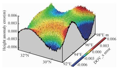
表5 Model3模型重建局部高程异常误差统计表(单位:m)Table 5 Error statistics of the reconstructed local height anomaly using Model3 (unit: m) |
| 统计量 | 数据量 | Max | Min | Mean | Std | Rms |
|---|---|---|---|---|---|---|
| ζ3300-ζ0+Δζ | 120×180 | 0.0058 | -0.0069 | -0.0005 | 0.0013 | 0.0014 |
表6 SHA方法延拓无噪声局部航空重力数据误差统计表Table 6 Error statistics table for downward continuation of noise-free local airborne gravity anomalies by SHA |
| 统计量 | 扣除边界大小 | 数据量 | Max | Min | Mean | Std | Rms |
|---|---|---|---|---|---|---|---|
| ΔgModel40-Δg0/mGal | 0° | 240×300 | 116.462 | -25.488 | 0.0007 | 4.147 | 4.147 |
| 0.5° | 210×270 | 8.308 | -8.135 | -0.003 | 0.704 | 0.704 | |
| 1.0° | 180×240 | 4.031 | -3.907 | -0.001 | 0.538 | 0.538 | |
| 2.0° | 120×180 | 1.793 | -1.893 | -0.002 | 0.413 | 0.413 |
表7 SHA方法向下延拓具有3 mGal噪声的局部航空重力数据误差统计表Table 7 Error statistics table for downward continuation of local airborne gravity anomalies with 3 mGal noise by SHA |
| 统计量 | 截断阶次 | Max | Min | Mean | Std | Rms |
|---|---|---|---|---|---|---|
| ΔgModel50-Δg0/mGal | 5400 | 68.259 | -68.791 | -0.028 | 17.520 | 17.519 |
| ΔgModel50(4320)-Δg0/mGal | 4320 | 51.176 | -53.418 | -0.027 | 10.581 | 10.580 |
| ΔgModel50(3600)-Δg0/mGal | 3600 | 67.196 | -72.251 | -0.029 | 9.747 | 9.747 |
| ΔgModel50(3240)-Δg0/mGal | 3240 | 76.301 | -88.343 | -0.030 | 10.112 | 10.112 |
表8 截断至2160阶的SHA方法向下延拓具有3 mGal噪声的航空重力数据的误差统计表Table 8 Error statistics table for downward continuation of local airborne gravity anomalies with 3 mGal noise by SHA truncated to 2160 degree |
| 统计量 | Max | Min | Mean | Std | Rms |
|---|---|---|---|---|---|
| ΔgModel60(2160)-Δg0/mGal | 7.815 | -7.795 | -0.027 | 2.061 | 2.061 |
| ΔgModel70(2160)-Δg0/mGal | 7.603 | -8.349 | -0.152 | 2.117 | 2.122 |
感谢审稿专家提出的修改意见和编辑部的大力支持!
|
|
|
|
|
|
|
|
|
Flechtner F, Dahle C, Neumayer K H, et al. 2010. The release 04 CHAMP and GRACE EIGEN gravity field models. //Flechtner F M, Gruber T, Güntner A, et al eds. System Earth via Geodetic-Geophysical Space Techniques. Berlin, Heidelberg: Springer, 41 -58.
|
|
|
|
|
|
|
|
|
|
Hofmann-Wellenhof B, Moritz H. 2006. Physical Geodesy. 2nd ed. Vienna: Springer.
|
|
|
|
|
|
|
|
|
|
|
|
|
|
|
|
Li X X. 2013. Building of an ultra-high-degree geopotential model [Master's thesis](in Chinese). Zhengzhou: PLA Information Engineering University.
|
|
Liang W, Xu X Y, Li J C, et al. 2023. Research on determination of gravity field models in regional area using airborne gravity data and reference model. Geomatics and Information Science of Wuhan University (in Chinese). https://doi.org/10.13203/j.whugis20230002.
|
|
|
|
|
|
|
|
|
|
|
|
|
|
|
|
|
|
|
|
|
|
|
|
|
|
|
|
|
|
|
|
|
|
|
|
|
|
|
|
|
|
|
|
|
|
|
|
|
|
|
|
|
|
|
|
|
|
|
|
|
|
李新星. 2013. 超高阶地球重力场模型的构建[硕士论文]. 郑州: 解放军信息工程大学.
|
|
梁伟, 徐新禹, 李建成, 等. 2023. 联合先验模型和航空重力数据构建适用于局部区域的超高阶重力场模型. 武汉大学学报(信息科学版), https://doi.org/10.13203/j.whugis20230002.
|
|
|
|
|
|
|
|
|
|
|
|
|
|
|
|
|
|
|
|
|
|
|
|
|
|
|
|
|
|
|
/
| 〈 |
|
〉 |


